Open-Source AI Cookbook documentation
用自定义数据集微调目标检测模型🖼,部署至 Spaces,并进行 Gradio API 集成
用自定义数据集微调目标检测模型🖼,部署至 Spaces,并进行 Gradio API 集成
在本 Notebook 中,我们将微调一个 目标检测 模型——具体来说是 DETR——使用一个自定义数据集。我们将利用 Hugging Face 生态系统 来完成此任务。
我们的做法是从一个预训练的 DETR 模型开始,并在一个标注的时尚图像自定义数据集上对其进行微调,即 Fashionpedia。通过这种方式,我们将调整模型,使其更好地识别和检测时尚领域中的物体。
在成功微调模型后,我们将把它部署为 Hugging Face 上的 Gradio Space。此外,我们还将探索如何通过 Gradio API 与部署的模型进行交互,实现与托管的 Space 之间的无缝通信,并为现实世界应用解锁新的可能性。

1. 安装依赖项
首先,我们需要安装用于微调目标检测模型的必要库。
!pip install -U -q datasets transformers[torch] timm wandb torchmetrics matplotlib albumentations
# Tested with datasets==2.21.0, transformers==4.44.2 timm==1.0.9, wandb==0.17.9 torchmetrics==1.4.1
2. 加载数据集 📁
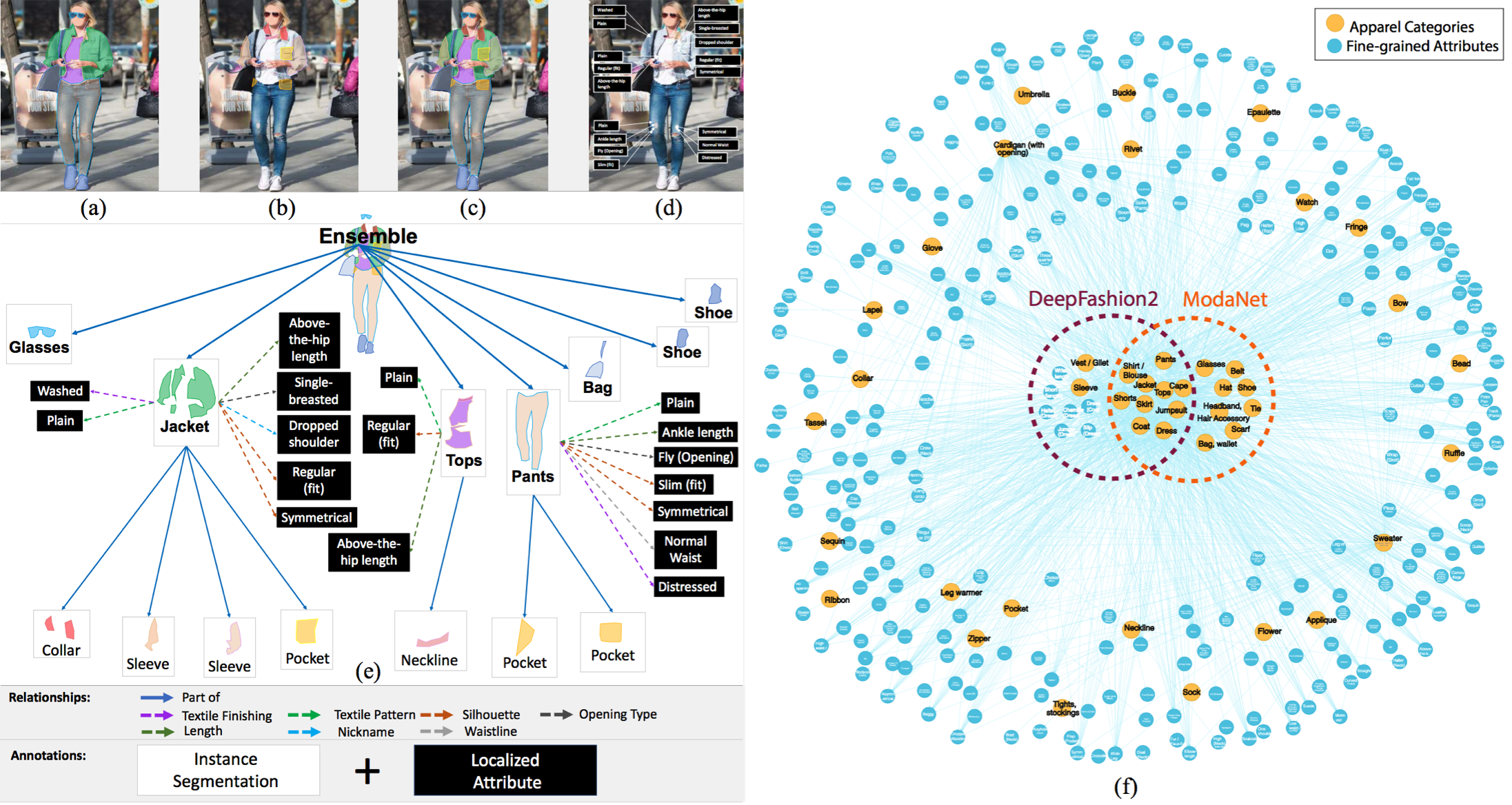
📁 我们将使用的数据集是 Fashionpedia,该数据集来源于论文 Fashionpedia: Ontology, Segmentation, and an Attribute Localization Dataset。作者对其描述如下:
Fashionpedia 是一个包含两部分的数据集:(1)由时尚专家构建的本体,包含27个主要服装类别、19个服装部件、294个细粒度属性及其关系;(2)一个包含48,000张日常生活和名人活动时尚图像的数据集,这些图像使用分割掩膜进行了标注,并附有每个掩膜的细粒度属性,基于 Fashionpedia 本体构建。该数据集包括:
- 46,781 张图像 🖼
- 342,182 个边界框 📦
它可以在 Hugging Face 上获取:Fashionpedia 数据集
from datasets import load_dataset

dataset = load_dataset("detection-datasets/fashionpedia")dataset
审查一个示例的内部结构
dataset["train"][0]3. 获取数据集的训练集和测试集拆分 ➗
该数据集包含两个拆分:训练集和测试集。我们将使用训练集来微调模型,使用测试集进行验证。
train_dataset = dataset["train"]
test_dataset = dataset["val"]
可选
在接下来的注释单元格中,我们从原始数据集中随机抽取了 1% 的样本用于训练集和测试集。这种方法用于加速训练过程,因为数据集包含大量示例。
为了获得最佳结果,建议跳过这两个单元格并使用完整数据集。 但如果需要,你可以取消注释这些单元格。
"""
def create_sample(dataset, sample_fraction=0.01, seed=42):
    sample_size = int(sample_fraction * len(dataset))
    sampled_dataset = dataset.shuffle(seed=seed).select(range(sample_size))
    print(f"Original size: {len(dataset)}")
    print(f"Sample size: {len(sampled_dataset)}")
    return sampled_dataset

# Apply function to both splits
train_dataset = create_sample(train_dataset)
test_dataset = create_sample(test_dataset)
"""
4. 可视化数据集中的一个示例及其物体 👀
现在我们已经加载了数据集,让我们可视化一个示例图像及其标注的物体。
生成 id2label 和 label2id
这两个变量包含物体 ID 与其对应标签之间的映射关系。id2label 将 ID 映射到标签,而 label2id 则将标签映射到 ID。
import numpy as np
from PIL import Image, ImageDraw


id2label = {
    0: "shirt, blouse",
    1: "top, t-shirt, sweatshirt",
    2: "sweater",
    3: "cardigan",
    4: "jacket",
    5: "vest",
    6: "pants",
    7: "shorts",
    8: "skirt",
    9: "coat",
    10: "dress",
    11: "jumpsuit",
    12: "cape",
    13: "glasses",
    14: "hat",
    15: "headband, head covering, hair accessory",
    16: "tie",
    17: "glove",
    18: "watch",
    19: "belt",
    20: "leg warmer",
    21: "tights, stockings",
    22: "sock",
    23: "shoe",
    24: "bag, wallet",
    25: "scarf",
    26: "umbrella",
    27: "hood",
    28: "collar",
    29: "lapel",
    30: "epaulette",
    31: "sleeve",
    32: "pocket",
    33: "neckline",
    34: "buckle",
    35: "zipper",
    36: "applique",
    37: "bead",
    38: "bow",
    39: "flower",
    40: "fringe",
    41: "ribbon",
    42: "rivet",
    43: "ruffle",
    44: "sequin",
    45: "tassel",
}


label2id = {v: k for k, v in id2label.items()}
我们来绘制一张图像! 🎨
现在,让我们从数据集中可视化一张图像,以便更好地了解它的样子。
>>> def draw_image_from_idx(dataset, idx):
...     sample = dataset[idx]
...     image = sample["image"]
...     annotations = sample["objects"]
...     draw = ImageDraw.Draw(image)
...     width, height = sample["width"], sample["height"]

...     print(annotations)

...     for i in range(len(annotations["bbox_id"])):
...         box = annotations["bbox"][i]
...         x1, y1, x2, y2 = tuple(box)
...         draw.rectangle((x1, y1, x2, y2), outline="red", width=3)
...         draw.text((x1, y1), id2label[annotations["category"][i]], fill="green")

...     return image


>>> draw_image_from_idx(dataset=train_dataset, idx=10)  # You can test changing this id
{'bbox_id': [158977, 158978, 158979, 158980, 158981, 158982, 158983], 'category': [1, 23, 23, 6, 31, 31, 33], 'bbox': [[210.0, 225.0, 536.0, 784.0], [290.0, 897.0, 350.0, 1015.0], [464.0, 950.0, 534.0, 1021.0], [313.0, 407.0, 524.0, 954.0], [268.0, 229.0, 333.0, 563.0], [489.0, 247.0, 528.0, 591.0], [387.0, 225.0, 450.0, 253.0]], 'area': [69960, 2449, 1788, 75418, 15149, 5998, 479]}
让我们可视化更多图像 📸
现在,让我们看几张来自数据集的图像,以便更全面地了解数据。
>>> import matplotlib.pyplot as plt


>>> def plot_images(dataset, indices):
...     """
...     Plot images and their annotations.
...     """
...     num_cols = 3
...     num_rows = int(np.ceil(len(indices) / num_cols))
...     fig, axes = plt.subplots(num_rows, num_cols, figsize=(15, 10))

...     for i, idx in enumerate(indices):
...         row = i // num_cols
...         col = i % num_cols

...         image = draw_image_from_idx(dataset, idx)

...         axes[row, col].imshow(image)
...         axes[row, col].axis("off")

...     for j in range(i + 1, num_rows * num_cols):
...         fig.delaxes(axes.flatten()[j])

...     plt.tight_layout()
...     plt.show()


>>> plot_images(train_dataset, range(9))
{'bbox_id': [150311, 150312, 150313, 150314], 'category': [23, 23, 33, 10], 'bbox': [[445.0, 910.0, 505.0, 983.0], [239.0, 940.0, 284.0, 994.0], [298.0, 282.0, 386.0, 352.0], [210.0, 282.0, 448.0, 665.0]], 'area': [1422, 843, 373, 56375]} {'bbox_id': [158953, 158954, 158955, 158956, 158957, 158958, 158959, 158960, 158961, 158962], 'category': [2, 33, 31, 31, 13, 7, 22, 22, 23, 23], 'bbox': [[182.0, 220.0, 472.0, 647.0], [294.0, 221.0, 407.0, 257.0], [405.0, 297.0, 472.0, 647.0], [182.0, 264.0, 266.0, 621.0], [284.0, 135.0, 372.0, 169.0], [238.0, 537.0, 414.0, 606.0], [351.0, 732.0, 417.0, 922.0], [202.0, 749.0, 270.0, 930.0], [200.0, 921.0, 256.0, 979.0], [373.0, 903.0, 455.0, 966.0]], 'area': [87267, 1220, 16895, 18541, 1468, 9360, 8629, 8270, 2717, 3121]} {'bbox_id': [169196, 169197, 169198, 169199, 169200, 169201, 169202, 169203, 169204, 169205, 169206, 169207, 169208, 169209, 169210], 'category': [13, 29, 28, 32, 32, 31, 31, 0, 31, 31, 18, 4, 6, 23, 23], 'bbox': [[441.0, 132.0, 499.0, 150.0], [412.0, 164.0, 494.0, 295.0], [427.0, 164.0, 476.0, 207.0], [406.0, 326.0, 448.0, 335.0], [484.0, 327.0, 508.0, 334.0], [366.0, 323.0, 395.0, 372.0], [496.0, 271.0, 523.0, 302.0], [366.0, 164.0, 523.0, 372.0], [360.0, 186.0, 406.0, 332.0], [502.0, 201.0, 534.0, 321.0], [496.0, 259.0, 515.0, 278.0], [360.0, 164.0, 534.0, 411.0], [403.0, 384.0, 510.0, 638.0], [393.0, 584.0, 430.0, 663.0], [449.0, 638.0, 518.0, 681.0]], 'area': [587, 2922, 931, 262, 111, 1171, 540, 3981, 4457, 1724, 188, 26621, 16954, 2167, 1773]} {'bbox_id': [167967, 167968, 167969, 167970, 167971, 167972, 167973, 167974, 167975, 167976, 167977, 167978, 167979, 167980, 167981, 167982, 167983, 167984, 167985, 167986, 167987, 167988, 167989, 167990, 167991, 167992, 167993, 167994, 167995, 167996, 167997, 167998, 167999, 168000, 168001, 168002, 168003, 168004, 168005, 168006, 168007, 168008, 168009, 168010, 168011, 168012, 168013, 168014, 168015, 168016, 168017, 168018, 168019, 168020, 168021, 168022, 168023, 168024, 168025, 168026, 168027, 168028, 168029, 168030, 168031, 168032, 168033, 168034, 168035, 168036, 168037, 168038, 168039, 168040], 'category': [6, 23, 23, 31, 31, 4, 1, 35, 32, 35, 35, 35, 35, 28, 35, 42, 42, 42, 42, 42, 42, 42, 42, 42, 42, 42, 42, 42, 42, 42, 42, 42, 42, 42, 42, 42, 42, 42, 42, 42, 42, 42, 42, 42, 42, 42, 42, 42, 42, 42, 42, 42, 42, 42, 42, 42, 42, 42, 42, 42, 42, 42, 42, 42, 42, 42, 42, 42, 42, 42, 42, 42, 42, 33], 'bbox': [[300.0, 421.0, 460.0, 846.0], [383.0, 841.0, 432.0, 899.0], [304.0, 740.0, 347.0, 831.0], [246.0, 222.0, 295.0, 505.0], [456.0, 229.0, 492.0, 517.0], [246.0, 169.0, 492.0, 517.0], [355.0, 213.0, 450.0, 433.0], [289.0, 353.0, 303.0, 427.0], [442.0, 288.0, 460.0, 340.0], [451.0, 290.0, 458.0, 304.0], [407.0, 238.0, 473.0, 486.0], [487.0, 501.0, 491.0, 517.0], [246.0, 455.0, 252.0, 505.0], [340.0, 169.0, 442.0, 238.0], [348.0, 230.0, 372.0, 476.0], [411.0, 179.0, 414.0, 182.0], [414.0, 183.0, 418.0, 186.0], [418.0, 187.0, 421.0, 190.0], [421.0, 192.0, 425.0, 195.0], [424.0, 196.0, 428.0, 199.0], [426.0, 200.0, 430.0, 204.0], [429.0, 204.0, 433.0, 208.0], [431.0, 209.0, 435.0, 213.0], [433.0, 214.0, 437.0, 218.0], [434.0, 218.0, 438.0, 222.0], [436.0, 223.0, 440.0, 226.0], [437.0, 227.0, 441.0, 231.0], [438.0, 232.0, 442.0, 235.0], [433.0, 232.0, 437.0, 236.0], [429.0, 233.0, 432.0, 237.0], [423.0, 233.0, 426.0, 237.0], [417.0, 233.0, 421.0, 237.0], [353.0, 172.0, 355.0, 174.0], [353.0, 175.0, 354.0, 177.0], [351.0, 178.0, 353.0, 181.0], [350.0, 182.0, 351.0, 184.0], [347.0, 187.0, 350.0, 189.0], [346.0, 190.0, 349.0, 193.0], [345.0, 194.0, 348.0, 197.0], [344.0, 199.0, 347.0, 202.0], [342.0, 204.0, 346.0, 207.0], [342.0, 208.0, 345.0, 211.0], [342.0, 212.0, 344.0, 215.0], [342.0, 217.0, 345.0, 220.0], [344.0, 221.0, 346.0, 224.0], [348.0, 222.0, 350.0, 225.0], [353.0, 223.0, 356.0, 226.0], [359.0, 223.0, 361.0, 226.0], [364.0, 223.0, 366.0, 226.0], [247.0, 448.0, 253.0, 454.0], [251.0, 454.0, 254.0, 456.0], [252.0, 460.0, 255.0, 463.0], [252.0, 466.0, 255.0, 469.0], [253.0, 471.0, 255.0, 475.0], [253.0, 478.0, 255.0, 481.0], [253.0, 483.0, 256.0, 486.0], [254.0, 489.0, 256.0, 492.0], [254.0, 495.0, 256.0, 497.0], [247.0, 457.0, 249.0, 460.0], [247.0, 463.0, 249.0, 466.0], [248.0, 469.0, 249.0, 471.0], [248.0, 476.0, 250.0, 478.0], [248.0, 481.0, 250.0, 483.0], [249.0, 486.0, 250.0, 488.0], [487.0, 459.0, 490.0, 461.0], [487.0, 465.0, 490.0, 467.0], [487.0, 471.0, 490.0, 472.0], [487.0, 476.0, 489.0, 478.0], [486.0, 482.0, 489.0, 484.0], [486.0, 488.0, 489.0, 490.0], [486.0, 494.0, 488.0, 496.0], [486.0, 500.0, 488.0, 501.0], [485.0, 505.0, 487.0, 507.0], [365.0, 213.0, 409.0, 226.0]], 'area': [44062, 2140, 2633, 9206, 5905, 44791, 12948, 211, 335, 43, 691, 62, 104, 2169, 439, 9, 10, 9, 8, 9, 14, 10, 13, 13, 11, 11, 10, 10, 12, 10, 10, 14, 4, 2, 4, 2, 5, 6, 7, 7, 8, 7, 6, 7, 5, 5, 7, 6, 5, 12, 5, 7, 8, 6, 6, 6, 4, 4, 6, 5, 2, 4, 4, 2, 6, 6, 3, 4, 6, 6, 4, 2, 4, 94]} {'bbox_id': [168041, 168042, 168043, 168044, 168045, 168046, 168047], 'category': [10, 32, 35, 31, 4, 29, 33], 'bbox': [[238.0, 309.0, 471.0, 1022.0], [234.0, 572.0, 331.0, 602.0], [235.0, 580.0, 324.0, 599.0], [119.0, 318.0, 343.0, 856.0], [111.0, 262.0, 518.0, 1022.0], [166.0, 262.0, 393.0, 492.0], [238.0, 309.0, 278.0, 324.0]], 'area': [12132, 1548, 755, 43926, 178328, 9316, 136]} {'bbox_id': [160050, 160051, 160052, 160053, 160054, 160055], 'category': [10, 31, 31, 23, 23, 33], 'bbox': [[290.0, 364.0, 429.0, 665.0], [304.0, 369.0, 397.0, 508.0], [290.0, 468.0, 310.0, 522.0], [213.0, 842.0, 294.0, 905.0], [446.0, 840.0, 536.0, 896.0], [311.0, 364.0, 354.0, 379.0]], 'area': [26873, 5301, 747, 1438, 1677, 71]} {'bbox_id': [160056, 160057, 160058, 160059, 160060, 160061, 160062, 160063, 160064, 160065, 160066], 'category': [10, 36, 42, 42, 42, 42, 42, 42, 42, 23, 33], 'bbox': [[127.0, 198.0, 451.0, 949.0], [277.0, 336.0, 319.0, 402.0], [340.0, 343.0, 344.0, 347.0], [321.0, 338.0, 327.0, 343.0], [336.0, 361.0, 342.0, 365.0], [329.0, 321.0, 333.0, 326.0], [313.0, 294.0, 319.0, 300.0], [330.0, 299.0, 334.0, 304.0], [295.0, 330.0, 300.0, 334.0], [332.0, 926.0, 376.0, 946.0], [284.0, 198.0, 412.0, 270.0]], 'area': [137575, 1915, 14, 24, 18, 15, 25, 16, 16, 740, 586]} {'bbox_id': [158963, 158964, 158965, 158966, 158967, 158968, 158969, 158970, 158971], 'category': [1, 31, 31, 7, 22, 22, 23, 23, 33], 'bbox': [[262.0, 449.0, 435.0, 686.0], [399.0, 471.0, 435.0, 686.0], [262.0, 451.0, 294.0, 662.0], [276.0, 603.0, 423.0, 726.0], [291.0, 759.0, 343.0, 934.0], [341.0, 749.0, 401.0, 947.0], [302.0, 919.0, 337.0, 994.0], [323.0, 925.0, 374.0, 1005.0], [343.0, 456.0, 366.0, 467.0]], 'area': [22330, 4422, 4846, 14000, 6190, 6997, 1547, 2107, 49]} {'bbox_id': [158972, 158973, 158974, 158975, 158976], 'category': [23, 23, 28, 10, 5], 'bbox': [[412.0, 588.0, 451.0, 631.0], [333.0, 585.0, 357.0, 627.0], [361.0, 243.0, 396.0, 257.0], [303.0, 243.0, 447.0, 517.0], [330.0, 259.0, 425.0, 324.0]], 'area': [949, 737, 133, 17839, 2916]}
5. 过滤无效的边界框 ❌
作为数据预处理的第一步,我们将过滤掉一些无效的边界框。在审查数据集后,我们发现某些边界框没有有效的结构。因此,我们将丢弃这些无效的条目。
>>> from datasets import Dataset


>>> def filter_invalid_bboxes(example):
...     valid_bboxes = []
...     valid_bbox_ids = []
...     valid_categories = []
...     valid_areas = []

...     for i, bbox in enumerate(example["objects"]["bbox"]):
...         x_min, y_min, x_max, y_max = bbox[:4]
...         if x_min < x_max and y_min < y_max:
...             valid_bboxes.append(bbox)
...             valid_bbox_ids.append(example["objects"]["bbox_id"][i])
...             valid_categories.append(example["objects"]["category"][i])
...             valid_areas.append(example["objects"]["area"][i])
...         else:
...             print(
...                 f"Image with invalid bbox: {example['image_id']} Invalid bbox detected and discarded: {bbox} - bbox_id: {example['objects']['bbox_id'][i]} - category: {example['objects']['category'][i]}"
...             )

...     example["objects"]["bbox"] = valid_bboxes
...     example["objects"]["bbox_id"] = valid_bbox_ids
...     example["objects"]["category"] = valid_categories
...     example["objects"]["area"] = valid_areas

...     return example


>>> train_dataset = train_dataset.map(filter_invalid_bboxes)
>>> test_dataset = test_dataset.map(filter_invalid_bboxes)
Image with invalid bbox: 8396 Invalid bbox detected and discarded: [0.0, 0.0, 0.0, 0.0] - bbox_id: 139952 - category: 42 Image with invalid bbox: 19725 Invalid bbox detected and discarded: [0.0, 0.0, 0.0, 0.0] - bbox_id: 23298 - category: 42 Image with invalid bbox: 19725 Invalid bbox detected and discarded: [0.0, 0.0, 0.0, 0.0] - bbox_id: 23299 - category: 42 Image with invalid bbox: 21696 Invalid bbox detected and discarded: [0.0, 0.0, 0.0, 0.0] - bbox_id: 277148 - category: 42 Image with invalid bbox: 23055 Invalid bbox detected and discarded: [0.0, 0.0, 0.0, 0.0] - bbox_id: 287029 - category: 33 Image with invalid bbox: 23671 Invalid bbox detected and discarded: [0.0, 0.0, 0.0, 0.0] - bbox_id: 290142 - category: 42 Image with invalid bbox: 26549 Invalid bbox detected and discarded: [0.0, 0.0, 0.0, 0.0] - bbox_id: 311943 - category: 37 Image with invalid bbox: 26834 Invalid bbox detected and discarded: [0.0, 0.0, 0.0, 0.0] - bbox_id: 309141 - category: 37 Image with invalid bbox: 31748 Invalid bbox detected and discarded: [0.0, 0.0, 0.0, 0.0] - bbox_id: 262063 - category: 42 Image with invalid bbox: 34253 Invalid bbox detected and discarded: [0.0, 0.0, 0.0, 0.0] - bbox_id: 315750 - category: 19
>>> print(train_dataset)
>>> print(test_dataset)
Dataset({
features: ['image_id', 'image', 'width', 'height', 'objects'],
num_rows: 45623
})
Dataset({
features: ['image_id', 'image', 'width', 'height', 'objects'],
num_rows: 1158
})
6. 可视化类别分布 👀
让我们通过绘制每个类别的出现次数来进一步探索数据集。这将帮助我们了解类别的分布情况,并识别任何潜在的偏差。
id_list = []
category_examples = {}
for example in train_dataset:
    id_list += example["objects"]["bbox_id"]
    for category in example["objects"]["category"]:
        if id2label[category] not in category_examples:
            category_examples[id2label[category]] = 1
        else:
            category_examples[id2label[category]] += 1

id_list.sort()>>> import matplotlib.pyplot as plt
>>> categories = list(category_examples.keys())
>>> values = list(category_examples.values())
>>> fig, ax = plt.subplots(figsize=(12, 8))
>>> bars = ax.bar(categories, values, color="skyblue")
>>> ax.set_xlabel("Categories", fontsize=14)
>>> ax.set_ylabel("Number of Occurrences", fontsize=14)
>>> ax.set_title("Number of Occurrences by Category", fontsize=16)
>>> ax.set_xticklabels(categories, rotation=90, ha="right")
>>> ax.grid(axis="y", linestyle="--", alpha=0.7)
>>> for bar in bars:
... height = bar.get_height()
... ax.text(bar.get_x() + bar.get_width() / 2.0, height, f"{height}", ha="center", va="bottom", fontsize=10)
>>> plt.tight_layout()
>>> plt.show()
我们可以观察到,某些类别,如“鞋子”或“袖子”,在数据集中出现的频率较高。这表明数据集可能存在类别不平衡的情况,某些类别的出现频率远高于其他类别。识别这些不平衡对于解决模型训练中的潜在偏差至关重要。
7. 为数据集添加数据增强
数据增强 🪄 在目标检测任务中对于提高性能至关重要。在本节中,我们将利用 Albumentations 的功能来有效地增强我们的数据集。
Albumentations 提供了一系列强大的增强技术,专为目标检测量身定制。它允许进行各种转换,同时确保边界框得到准确调整。这些功能有助于生成更具多样性的数据集,提高模型的鲁棒性和泛化能力。
import albumentations as A

train_transform = A.Compose(
    [
        A.LongestMaxSize(500),
        A.PadIfNeeded(500, 500, border_mode=0, value=(0, 0, 0)),
        A.HorizontalFlip(p=0.5),
        A.RandomBrightnessContrast(p=0.5),
        A.HueSaturationValue(p=0.5),
        A.Rotate(limit=10, p=0.5),
        A.RandomScale(scale_limit=0.2, p=0.5),
        A.GaussianBlur(p=0.5),
        A.GaussNoise(p=0.5),
    ],
    bbox_params=A.BboxParams(format="pascal_voc", label_fields=["category"]),
)

val_transform = A.Compose(
    [
        A.LongestMaxSize(500),
        A.PadIfNeeded(500, 500, border_mode=0, value=(0, 0, 0)),
    ],
    bbox_params=A.BboxParams(format="pascal_voc", label_fields=["category"]),
)
8. 从模型检查点初始化图像处理器 🎆
我们将使用预训练的模型检查点来实例化图像处理器。在这种情况下,我们使用的是 facebook/detr-resnet-50-dc5 模型。
from transformers import AutoImageProcessor

checkpoint = "facebook/detr-resnet-50-dc5"
image_processor = AutoImageProcessor.from_pretrained(checkpoint)
添加处理数据集的方法
接下来,我们将添加方法来处理数据集。这些方法将处理图像和标注的转换任务,以确保它们与模型兼容。
def formatted_anns(image_id, category, area, bbox):
    annotations = []
    for i in range(0, len(category)):
        new_ann = {
            "image_id": image_id,
            "category_id": category[i],
            "isCrowd": 0,
            "area": area[i],
            "bbox": list(bbox[i]),
        }
        annotations.append(new_ann)

    return annotations


def convert_voc_to_coco(bbox):
    xmin, ymin, xmax, ymax = bbox
    width = xmax - xmin
    height = ymax - ymin
    return [xmin, ymin, width, height]


def transform_aug_ann(examples, transform):
    image_ids = examples["image_id"]
    images, bboxes, area, categories = [], [], [], []
    for image, objects in zip(examples["image"], examples["objects"]):
        image = np.array(image.convert("RGB"))[:, :, ::-1]
        out = transform(image=image, bboxes=objects["bbox"], category=objects["category"])

        area.append(objects["area"])
        images.append(out["image"])

        # Convert to COCO format
        converted_bboxes = [convert_voc_to_coco(bbox) for bbox in out["bboxes"]]
        bboxes.append(converted_bboxes)

        categories.append(out["category"])

    targets = [
        {"image_id": id_, "annotations": formatted_anns(id_, cat_, ar_, box_)}
        for id_, cat_, ar_, box_ in zip(image_ids, categories, area, bboxes)
    ]

    return image_processor(images=images, annotations=targets, return_tensors="pt")


def transform_train(examples):
    return transform_aug_ann(examples, transform=train_transform)


def transform_val(examples):
    return transform_aug_ann(examples, transform=val_transform)


train_dataset_transformed = train_dataset.with_transform(transform_train)
test_dataset_transformed = test_dataset.with_transform(transform_val)
9. 绘制增强后的示例 🎆
我们即将进入模型训练阶段!在继续之前,让我们可视化一些增强后的样本。这将帮助我们再次确认这些增强方法是否适合且有效,为训练过程做好准备。
>>> # Updated draw function to accept an optional transform
>>> def draw_augmented_image_from_idx(dataset, idx, transform=None):
...     sample = dataset[idx]
...     image = sample["image"]
...     annotations = sample["objects"]

...     # Convert image to RGB and NumPy array
...     image = np.array(image.convert("RGB"))[:, :, ::-1]

...     if transform:
...         augmented = transform(image=image, bboxes=annotations["bbox"], category=annotations["category"])
...         image = augmented["image"]
...         annotations["bbox"] = augmented["bboxes"]
...         annotations["category"] = augmented["category"]

...     image = Image.fromarray(image[:, :, ::-1])  # Convert back to PIL Image
...     draw = ImageDraw.Draw(image)
...     width, height = sample["width"], sample["height"]

...     for i in range(len(annotations["bbox_id"])):
...         box = annotations["bbox"][i]
...         x1, y1, x2, y2 = tuple(box)

...         # Normalize coordinates if necessary
...         if max(box) <= 1.0:
...             x1, y1 = int(x1 * width), int(y1 * height)
...             x2, y2 = int(x2 * width), int(y2 * height)
...         else:
...             x1, y1 = int(x1), int(y1)
...             x2, y2 = int(x2), int(y2)

...         draw.rectangle((x1, y1, x2, y2), outline="red", width=3)
...         draw.text((x1, y1), id2label[annotations["category"][i]], fill="green")

...     return image


>>> # Updated plot function to include augmentation
>>> def plot_augmented_images(dataset, indices, transform=None):
...     """
...     Plot images and their annotations with optional augmentation.
...     """
...     num_rows = len(indices) // 3
...     num_cols = 3
...     fig, axes = plt.subplots(num_rows, num_cols, figsize=(15, 10))

...     for i, idx in enumerate(indices):
...         row = i // num_cols
...         col = i % num_cols

...         # Draw augmented image
...         image = draw_augmented_image_from_idx(dataset, idx, transform=transform)

...         # Display image on the corresponding subplot
...         axes[row, col].imshow(image)
...         axes[row, col].axis("off")

...     plt.tight_layout()
...     plt.show()


>>> # Now use the function to plot augmented images
>>> plot_augmented_images(train_dataset, range(9), transform=train_transform)
10. 从检查点初始化模型
我们将使用与图像处理器相同的检查点来初始化模型。这包括加载一个预训练模型,我们将对其进行微调,以适应我们的特定数据集。
from transformers import AutoModelForObjectDetection

model = AutoModelForObjectDetection.from_pretrained(
    checkpoint,
    id2label=id2label,
    label2id=label2id,
    ignore_mismatched_sizes=True,
)output_dir = "detr-resnet-50-dc5-fashionpedia-finetuned" # change this11. 连接到 HF Hub 上传微调后的模型 🔌
我们将连接到 Hugging Face Hub 以上传我们的微调模型。这使我们能够共享和部署模型,供他人使用或进行进一步评估。
from huggingface_hub import notebook_login

notebook_login()
12. 设置训练参数,连接到 W&B,并开始训练!
接下来,我们将设置训练参数,连接到 Weights & Biases (W&B),并启动训练过程。W&B 将帮助我们跟踪实验、可视化指标,并管理我们的模型训练工作流。
from transformers import TrainingArguments
from transformers import Trainer

import torch

# Define the training arguments

training_args = TrainingArguments(
    output_dir=output_dir,
    per_device_train_batch_size=4,
    per_device_eval_batch_size=4,
    max_steps=10000,
    fp16=True,
    save_steps=10,
    logging_steps=1,
    learning_rate=1e-5,
    weight_decay=1e-4,
    save_total_limit=2,
    remove_unused_columns=False,
    evaluation_strategy="steps",
    eval_steps=50,
    eval_strategy="steps",
    report_to="wandb",
    push_to_hub=True,
    batch_eval_metrics=True,
)
连接到 W&B 跟踪训练
import wandb

wandb.init(
    project="detr-resnet-50-dc5-fashionpedia-finetuned",  # change this
    name="detr-resnet-50-dc5-fashionpedia-finetuned",  # change this
    config=training_args,
)
让我们开始训练模型! 🚀
现在是时候开始训练模型了。让我们运行训练过程,看看我们的微调模型如何从数据中学习!
首先,我们声明 compute_metrics 方法,用于在评估时计算指标。
from torchmetrics.detection.mean_ap import MeanAveragePrecision
from torch.nn.functional import softmax


def denormalize_boxes(boxes, width, height):
    boxes = boxes.clone()
    boxes[:, 0] *= width  # xmin
    boxes[:, 1] *= height  # ymin
    boxes[:, 2] *= width  # xmax
    boxes[:, 3] *= height  # ymax
    return boxes


batch_metrics = []


def compute_metrics(eval_pred, compute_result):
    global batch_metrics

    (loss_dict, scores, pred_boxes, last_hidden_state, encoder_last_hidden_state), labels = eval_pred

    image_sizes = []
    target = []
    for label in labels:

        image_sizes.append(label["orig_size"])
        width, height = label["orig_size"]
        denormalized_boxes = denormalize_boxes(label["boxes"], width, height)
        target.append(
            {
                "boxes": denormalized_boxes,
                "labels": label["class_labels"],
            }
        )
    predictions = []
    for score, box, target_sizes in zip(scores, pred_boxes, image_sizes):
        # Extract the bounding boxes, labels, and scores from the model's output
        pred_scores = score[:, :-1]  # Exclude the no-object class
        pred_scores = softmax(pred_scores, dim=-1)
        width, height = target_sizes
        pred_boxes = denormalize_boxes(box, width, height)
        pred_labels = torch.argmax(pred_scores, dim=-1)

        # Get the scores corresponding to the predicted labels
        pred_scores_for_labels = torch.gather(pred_scores, 1, pred_labels.unsqueeze(-1)).squeeze(-1)
        predictions.append(
            {
                "boxes": pred_boxes,
                "scores": pred_scores_for_labels,
                "labels": pred_labels,
            }
        )

    metric = MeanAveragePrecision(box_format="xywh", class_metrics=True)

    if not compute_result:
        # Accumulate batch-level metrics
        batch_metrics.append({"preds": predictions, "target": target})
        return {}
    else:
        # Compute final aggregated metrics
        # Aggregate batch-level metrics (this should be done based on your metric library's needs)
        all_preds = []
        all_targets = []
        for batch in batch_metrics:
            all_preds.extend(batch["preds"])
            all_targets.extend(batch["target"])

        # Update metric with all accumulated predictions and targets
        metric.update(preds=all_preds, target=all_targets)
        metrics = metric.compute()

        # Convert and format metrics as needed
        classes = metrics.pop("classes")
        map_per_class = metrics.pop("map_per_class")
        mar_100_per_class = metrics.pop("mar_100_per_class")

        for class_id, class_map, class_mar in zip(classes, map_per_class, mar_100_per_class):
            class_name = id2label[class_id.item()] if id2label is not None else class_id.item()
            metrics[f"map_{class_name}"] = class_map
            metrics[f"mar_100_{class_name}"] = class_mar

        # Round metrics for cleaner output
        metrics = {k: round(v.item(), 4) for k, v in metrics.items()}

        # Clear batch metrics for next evaluation
        batch_metrics = []

return metricsdef collate_fn(batch):
pixel_values = [item["pixel_values"] for item in batch]
encoding = image_processor.pad(pixel_values, return_tensors="pt")
labels = [item["labels"] for item in batch]
batch = {}
batch["pixel_values"] = encoding["pixel_values"]
batch["pixel_mask"] = encoding["pixel_mask"]
batch["labels"] = labels
return batchtrainer = Trainer(
model=model,
args=training_args,
data_collator=collate_fn,
train_dataset=train_dataset_transformed,
eval_dataset=test_dataset_transformed,
tokenizer=image_processor,
compute_metrics=compute_metrics,
)trainer.train()
trainer.push_to_hub()
13. 测试模型在测试图像上的表现 📝
模型训练完成后,我们可以评估其在测试图像上的表现。由于该模型已作为 Hugging Face 模型提供,因此进行预测非常简单。在接下来的单元格中,我们将展示如何在新图像上运行推理并评估模型的能力。
import requests
from transformers import pipeline
import numpy as np
from PIL import Image, ImageDraw

url = "https://images.unsplash.com/photo-1536243298747-ea8874136d64?q=80&w=640"

image = Image.open(requests.get(url, stream=True).raw)

obj_detector = pipeline(
    "object-detection", model="sergiopaniego/detr-resnet-50-dc5-fashionpedia-finetuned"  # Change with your model name
)


results = obj_detector(image)
print(results)
现在,让我们展示结果
我们将展示模型在测试图像上的预测结果。这将让我们了解模型的表现情况,并突出其优势和需要改进的地方。
from PIL import Image, ImageDraw
import numpy as np


def plot_results(image, results, threshold=0.6):
    image = Image.fromarray(np.uint8(image))
    draw = ImageDraw.Draw(image)
    width, height = image.size

    for result in results:
        score = result["score"]
        label = result["label"]
        box = list(result["box"].values())

        if score > threshold:
            x1, y1, x2, y2 = tuple(box)
            draw.rectangle((x1, y1, x2, y2), outline="red", width=3)
            draw.text((x1 + 5, y1 - 10), label, fill="white")
            draw.text((x1 + 5, y1 + 10), f"{score:.2f}", fill="green" if score > 0.7 else "red")

return image>>> plot_results(image, results)
14. 在测试集上评估模型 📝
在训练并可视化测试图像的结果后,我们将对整个测试数据集进行模型评估。这一步包括生成评估指标,以评估模型在所有测试样本上的整体表现和有效性。
metrics = trainer.evaluate(test_dataset_transformed)
print(metrics)
15. 将模型部署到 HF Space

现在我们的模型已经在 Hugging Face 上可用,我们可以将其部署到 HF Space。Hugging Face 为小型应用提供免费的 Spaces,使我们能够创建一个交互式网页应用,用户可以上传测试图像并评估模型的能力。
我已经在这里创建了一个示例应用:DETR 目标检测 Fashionpedia - 微调版
from IPython.display import IFrame

IFrame(src="https://sergiopaniego-detr-object-detection-fashionpedia-fa0081f.hf.space", width=1000, height=800)
使用以下代码创建应用
你可以通过将以下代码复制并粘贴到一个名为 app.py 的文件中来创建一个新应用。
# app.py

import gradio as gr
import spaces
import torch

from PIL import Image
from transformers import pipeline
import matplotlib.pyplot as plt
import io

model_pipeline = pipeline("object-detection", model="sergiopaniego/detr-resnet-50-dc5-fashionpedia-finetuned")


COLORS = [
    [0.000, 0.447, 0.741],
    [0.850, 0.325, 0.098],
    [0.929, 0.694, 0.125],
    [0.494, 0.184, 0.556],
    [0.466, 0.674, 0.188],
    [0.301, 0.745, 0.933],
]


def get_output_figure(pil_img, results, threshold):
    plt.figure(figsize=(16, 10))
    plt.imshow(pil_img)
    ax = plt.gca()
    colors = COLORS * 100

    for result in results:
        score = result["score"]
        label = result["label"]
        box = list(result["box"].values())
        if score > threshold:
            c = COLORS[hash(label) % len(COLORS)]
            ax.add_patch(
                plt.Rectangle((box[0], box[1]), box[2] - box[0], box[3] - box[1], fill=False, color=c, linewidth=3)
            )
            text = f"{label}: {score:0.2f}"
            ax.text(box[0], box[1], text, fontsize=15, bbox=dict(facecolor="yellow", alpha=0.5))
    plt.axis("off")

    return plt.gcf()


@spaces.GPU
def detect(image):
    results = model_pipeline(image)
    print(results)

    output_figure = get_output_figure(image, results, threshold=0.7)

    buf = io.BytesIO()
    output_figure.savefig(buf, bbox_inches="tight")
    buf.seek(0)
    output_pil_img = Image.open(buf)

    return output_pil_img


with gr.Blocks() as demo:
    gr.Markdown("# Object detection with DETR fine tuned on detection-datasets/fashionpedia")
    gr.Markdown(
        """
        This application uses a fine tuned DETR (DEtection TRansformers) to detect objects on images.
        This version was trained using detection-datasets/fashionpedia dataset.
        You can load an image and see the predictions for the objects detected.
        """
    )

    gr.Interface(
        fn=detect,
        inputs=gr.Image(label="Input image", type="pil"),
        outputs=[gr.Image(label="Output prediction", type="pil")],
    )

demo.launch(show_error=True)
别忘了设置 requirements.txt
不要忘记创建一个 requirements.txt 文件,以指定应用程序的依赖项。
!touch requirements.txt
!echo -e "transformers\ntimm\ntorch\ngradio\nmatplotlib" > requirements.txt
16. 将 Space 作为 API 访问 🧑💻️
Hugging Face Spaces 的一个优点是,它们提供了一个可以从外部应用程序访问的 API。这使得将模型集成到各种应用程序中变得非常容易,无论是使用 JavaScript、Python 还是其他语言开发的应用程序。想象一下扩展和利用模型功能的各种可能性!
你可以在这里找到更多关于如何使用 API 的信息:Hugging Face 企业指南:Gradio
!pip install gradio_client
from gradio_client import Client, handle_file

client = Client("sergiopaniego/DETR_object_detection_fashionpedia-finetuned")  # change this with your Space
result = client.predict(
    image=handle_file("https://images.unsplash.com/photo-1536243298747-ea8874136d64?q=80&w=640"), api_name="/predict"
)from PIL import Image
img = Image.open(result).convert("RGB")>>> from IPython.display import display
>>> display(img)
结论
在本教程中,我们成功地在自定义数据集上微调了一个目标检测模型,并将其部署为 Gradio Space。我们还演示了如何使用 Gradio API 调用该 Space,展示了将其集成到各种应用程序中的简便性。
希望本指南能帮助您自信地微调和部署自己的模型! 🚀
< > Update on GitHub