
File size: 68,542 Bytes
7934b29 |
1 2 3 4 5 6 7 8 9 10 11 12 13 14 15 16 17 18 19 20 21 22 23 24 25 26 27 28 29 30 31 32 33 34 35 36 37 38 39 40 41 42 43 44 45 46 47 48 49 50 51 52 53 54 55 56 57 58 59 60 61 62 63 64 65 66 67 68 69 70 71 72 73 74 75 76 77 78 79 80 81 82 83 84 85 86 87 88 89 90 91 92 93 94 95 96 97 98 99 100 101 102 103 104 105 106 107 108 109 110 111 112 113 114 115 116 117 118 119 120 121 122 123 124 125 126 127 128 129 130 131 132 133 134 135 136 137 138 139 140 141 142 143 144 145 146 147 148 149 150 151 152 153 154 155 156 157 158 159 160 161 162 163 164 165 166 167 168 169 170 171 172 173 174 175 176 177 178 179 180 181 182 183 184 185 186 187 188 189 190 191 192 193 194 195 196 197 198 199 200 201 202 203 204 205 206 207 208 209 210 211 212 213 214 215 216 217 218 219 220 221 222 223 224 225 226 227 228 229 230 231 232 233 234 235 236 237 238 239 240 241 242 243 244 245 246 247 248 249 250 251 252 253 254 255 256 257 258 259 260 261 262 263 264 265 266 267 268 269 270 271 272 273 274 275 276 277 278 279 280 281 282 283 284 285 286 287 288 289 290 291 292 293 294 295 296 297 298 299 300 301 302 303 304 305 306 307 308 309 310 311 312 313 314 315 316 317 318 319 320 321 322 323 324 325 326 327 328 329 330 331 332 333 334 335 336 337 338 339 340 341 342 343 344 345 346 347 348 349 350 351 352 353 354 355 356 357 358 359 360 361 362 363 364 365 366 367 368 369 370 371 372 373 374 375 376 377 378 379 380 381 382 383 384 385 386 387 388 389 390 391 392 393 394 395 396 397 398 399 400 401 402 403 404 405 406 407 408 409 410 411 412 413 414 415 416 417 418 419 420 421 422 423 424 425 426 427 428 429 430 431 432 433 434 435 436 437 438 439 440 441 442 443 444 445 446 447 448 449 450 451 452 453 454 455 456 457 458 459 460 461 462 463 464 465 466 467 468 469 470 471 472 473 474 475 476 477 478 479 480 481 482 483 484 485 486 487 488 489 490 491 492 493 494 495 496 497 498 499 500 501 502 503 504 505 506 507 508 509 510 511 512 513 514 515 516 517 518 519 520 521 522 523 524 525 526 527 528 529 530 531 532 533 534 535 536 537 538 539 540 541 542 543 544 545 546 547 548 549 550 551 552 553 554 555 556 557 558 559 560 561 562 563 564 565 566 567 568 569 570 571 572 573 574 575 576 577 578 579 580 581 582 583 584 585 586 587 588 589 590 591 592 593 594 595 596 597 598 599 600 601 602 603 604 605 606 607 608 609 610 611 612 613 614 615 616 617 618 619 620 621 622 623 624 625 626 627 628 629 630 631 632 633 634 635 636 637 638 639 640 641 642 643 644 645 646 647 648 649 650 651 652 653 654 655 656 657 658 659 660 661 662 663 664 665 666 667 668 669 670 671 672 673 674 675 676 677 678 679 680 681 682 683 684 685 686 687 688 689 690 691 692 693 694 695 696 697 698 699 700 701 702 703 704 705 706 707 708 709 710 711 712 713 714 715 716 717 718 719 720 721 722 723 724 725 726 727 728 729 730 731 732 733 734 735 736 737 738 739 740 741 742 743 744 745 746 747 748 749 750 751 752 753 754 755 756 757 758 759 760 761 762 763 764 765 766 767 768 769 770 771 772 773 774 775 776 777 778 779 780 781 782 783 784 785 786 787 788 789 790 791 792 793 794 795 796 797 798 799 800 801 802 803 804 805 806 807 808 809 810 811 812 813 814 815 816 817 818 819 820 821 822 823 824 825 826 827 828 829 830 831 832 833 834 835 836 837 838 839 840 841 842 843 844 845 846 847 848 849 850 851 852 853 854 855 856 857 858 859 860 861 862 863 864 865 866 867 868 869 870 871 872 873 874 875 876 877 878 879 880 881 882 883 884 885 886 887 888 889 890 891 892 893 894 895 896 897 898 899 900 901 902 903 904 905 906 907 908 909 910 911 912 913 914 915 916 917 918 919 920 921 922 923 924 925 926 927 928 929 930 931 932 933 934 935 936 937 938 939 940 941 942 943 944 945 946 947 948 949 950 951 952 953 954 955 956 957 958 959 960 961 962 963 964 965 966 967 968 969 970 971 972 973 974 975 976 977 978 979 980 981 982 983 984 985 986 987 988 989 990 991 992 993 994 995 996 997 998 999 1000 1001 1002 1003 1004 1005 1006 1007 1008 1009 1010 1011 1012 1013 1014 1015 1016 1017 1018 1019 1020 1021 1022 1023 1024 1025 1026 1027 1028 1029 1030 1031 1032 1033 1034 1035 1036 1037 1038 1039 1040 1041 1042 1043 1044 1045 1046 1047 1048 1049 1050 1051 1052 1053 1054 1055 1056 1057 1058 1059 1060 1061 1062 1063 1064 1065 1066 1067 1068 1069 1070 1071 1072 1073 1074 1075 1076 1077 1078 1079 1080 1081 1082 1083 1084 1085 1086 1087 1088 1089 1090 1091 1092 1093 1094 1095 1096 1097 1098 1099 1100 1101 1102 1103 1104 1105 1106 1107 1108 1109 1110 1111 1112 1113 1114 1115 1116 1117 1118 1119 1120 1121 1122 1123 1124 1125 1126 1127 1128 1129 1130 1131 1132 1133 1134 1135 1136 1137 1138 1139 1140 1141 1142 1143 1144 1145 1146 1147 1148 1149 1150 1151 1152 1153 1154 1155 1156 1157 1158 1159 1160 1161 1162 1163 1164 1165 1166 1167 1168 1169 1170 1171 1172 1173 1174 1175 1176 |
{
"nbformat": 4,
"nbformat_minor": 0,
"metadata": {
"accelerator": "GPU",
"colab": {
"name": "ASR_with_NeMo.ipynb",
"provenance": [],
"collapsed_sections": [],
"toc_visible": true
},
"kernelspec": {
"display_name": "Python 3",
"language": "python",
"name": "python3"
},
"language_info": {
"codemirror_mode": {
"name": "ipython",
"version": 3
},
"file_extension": ".py",
"mimetype": "text/x-python",
"name": "python",
"nbconvert_exporter": "python",
"pygments_lexer": "ipython3",
"version": "3.7.7"
}
},
"cells": [
{
"cell_type": "code",
"metadata": {
"id": "lJz6FDU1lRzc"
},
"source": [
"\"\"\"\n",
"You can run either this notebook locally (if you have all the dependencies and a GPU) or on Google Colab.\n",
"\n",
"Instructions for setting up Colab are as follows:\n",
"1. Open a new Python 3 notebook.\n",
"2. Import this notebook from GitHub (File -> Upload Notebook -> \"GITHUB\" tab -> copy/paste GitHub URL)\n",
"3. Connect to an instance with a GPU (Runtime -> Change runtime type -> select \"GPU\" for hardware accelerator)\n",
"4. Run this cell to set up dependencies.\n",
"5. Restart the runtime (Runtime -> Restart Runtime) for any upgraded packages to take effect\n",
"\"\"\"\n",
"# If you're using Google Colab and not running locally, run this cell.\n",
"\n",
"## Install dependencies\n",
"!pip install wget\n",
"!apt-get install sox libsndfile1 ffmpeg\n",
"!pip install text-unidecode\n",
"!pip install matplotlib>=3.3.2\n",
"\n",
"## Install NeMo\n",
"BRANCH = 'r1.17.0'\n",
"!python -m pip install git+https://github.com/NVIDIA/NeMo.git@$BRANCH#egg=nemo_toolkit[all]\n",
"\n",
"\"\"\"\n",
"Remember to restart the runtime for the kernel to pick up any upgraded packages (e.g. matplotlib)!\n",
"Alternatively, you can uncomment the exit() below to crash and restart the kernel, in the case\n",
"that you want to use the \"Run All Cells\" (or similar) option.\n",
"\"\"\"\n",
"# exit()"
],
"execution_count": null,
"outputs": []
},
{
"cell_type": "markdown",
"metadata": {
"id": "v1Jk9etFlRzf"
},
"source": [
"# Introduction to End-To-End Automatic Speech Recognition\n",
"\n",
"This notebook contains a basic tutorial of Automatic Speech Recognition (ASR) concepts, introduced with code snippets using the [NeMo framework](https://github.com/NVIDIA/NeMo).\n",
"We will first introduce the basics of the main concepts behind speech recognition, then explore concrete examples of what the data looks like and walk through putting together a simple end-to-end ASR pipeline.\n",
"\n",
"We assume that you are familiar with general machine learning concepts and can follow Python code, and we'll be using the [AN4 dataset from CMU](http://www.speech.cs.cmu.edu/databases/an4/) (with processing using `sox`)."
]
},
{
"cell_type": "markdown",
"metadata": {
"id": "YLln3U-IlRzg"
},
"source": [
"## Conceptual Overview: What is ASR?\n",
"\n",
"ASR, or **Automatic Speech Recognition**, refers to the problem of getting a program to automatically transcribe spoken language (speech-to-text). Our goal is usually to have a model that minimizes the **Word Error Rate (WER)** metric when transcribing speech input. In other words, given some audio file (e.g. a WAV file) containing speech, how do we transform this into the corresponding text with as few errors as possible?\n",
"\n",
"Traditional speech recognition takes a generative approach, modeling the full pipeline of how speech sounds are produced in order to evaluate a speech sample. We would start from a **language model** that encapsulates the most likely orderings of words that are generated (e.g. an n-gram model), to a **pronunciation model** for each word in that ordering (e.g. a pronunciation table), to an **acoustic model** that translates those pronunciations to audio waveforms (e.g. a Gaussian Mixture Model).\n",
"\n",
"Then, if we receive some spoken input, our goal would be to find the most likely sequence of text that would result in the given audio according to our generative pipeline of models. Overall, with traditional speech recognition, we try to model `Pr(audio|transcript)*Pr(transcript)`, and take the argmax of this over possible transcripts.\n",
"\n",
"Over time, neural nets advanced to the point where each component of the traditional speech recognition model could be replaced by a neural model that had better performance and that had a greater potential for generalization. For example, we could replace an n-gram model with a neural language model, and replace a pronunciation table with a neural pronunciation model, and so on. However, each of these neural models need to be trained individually on different tasks, and errors in any model in the pipeline could throw off the whole prediction.\n",
"\n",
"Thus, we can see the appeal of **end-to-end ASR architectures**: discriminative models that simply take an audio input and give a textual output, and in which all components of the architecture are trained together towards the same goal. The model's encoder would be akin to an acoustic model for extracting speech features, which can then be directly piped to a decoder which outputs text. If desired, we could integrate a language model that would improve our predictions, as well.\n",
"\n",
"And the entire end-to-end ASR model can be trained at once--a much easier pipeline to handle! "
]
},
{
"cell_type": "markdown",
"metadata": {
"id": "0S5iZPMSlRzg"
},
"source": [
"### End-To-End ASR\n",
"\n",
"With an end-to-end model, we want to directly learn `Pr(transcript|audio)` in order to predict the transcripts from the original audio. Since we are dealing with sequential information--audio data over time that corresponds to a sequence of letters--RNNs are the obvious choice. But now we have a pressing problem to deal with: since our input sequence (number of audio timesteps) is not the same length as our desired output (transcript length), how do we match each time step from the audio data to the correct output characters?\n",
"\n",
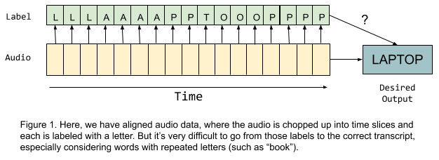
"Earlier speech recognition approaches relied on **temporally-aligned data**, in which each segment of time in an audio file was matched up to a corresponding speech sound such as a phoneme or word. However, if we would like to have the flexibility to predict letter-by-letter to prevent OOV (out of vocabulary) issues, then each time step in the data would have to be labeled with the letter sound that the speaker is making at that point in the audio file. With that information, it seems like we should simply be able to try to predict the correct letter for each time step and then collapse the repeated letters (e.g. the prediction output `LLLAAAAPPTOOOPPPP` would become `LAPTOP`). It turns out that this idea has some problems: not only does alignment make the dataset incredibly labor-intensive to label, but also, what do we do with words like \"book\" that contain consecutive repeated letters? Simply squashing repeated letters together would not work in that case!\n",
"\n",
"\n",
"\n",
"Modern end-to-end approaches get around this using methods that don't require manual alignment at all, so that the input-output pairs are really just the raw audio and the transcript--no extra data or labeling required. Let's briefly go over two popular approaches that allow us to do this, Connectionist Temporal Classification (CTC) and sequence-to-sequence models with attention.\n",
"\n",
"#### Connectionist Temporal Classification (CTC)\n",
"\n",
"In normal speech recognition prediction output, we would expect to have characters such as the letters from A through Z, numbers 0 through 9, spaces (\"\\_\"), and so on. CTC introduces a new intermediate output token called the **blank token** (\"-\") that is useful for getting around the alignment issue.\n",
"\n",
"With CTC, we still predict one token per time segment of speech, but we use the blank token to figure out where we can and can't collapse the predictions. The appearance of a blank token helps separate repeating letters that should not be collapsed. For instance, with an audio snippet segmented into `T=11` time steps, we could get predictions that look like `BOO-OOO--KK`, which would then collapse to `\"BO-O-K\"`, and then we would remove the blank tokens to get our final output, `BOOK`.\n",
"\n",
"Now, we can predict one output token per time step, then collapse and clean to get sensible output without any fear of ambiguity from repeating letters! A simple way of getting predictions like this would be to apply a bidirectional RNN to the audio input, apply softmax over each time step's output, and then take the token with the highest probability. The method of always taking the best token at each time step is called **greedy decoding, or max decoding**.\n",
"\n",
"To calculate our loss for backprop, we would like to know the log probability of the model producing the correct transcript, `log(Pr(transcript|audio))`. We can get the log probability of a single intermediate output sequence (e.g. `BOO-OOO--KK`) by summing over the log probabilities we get from each token's softmax value, but note that the resulting sum is different from the log probability of the transcript itself (`BOOK`). This is because there are multiple possible output sequences of the same length that can be collapsed to get the same transcript (e.g. `BBO--OO-KKK` also results in `BOOK`), and so we need to **marginalize over every valid sequence of length `T` that collapses to the transcript**.\n",
"\n",
"Therefore, to get our transcript's log probability given our audio input, we must sum the log probabilities of every sequence of length `T` that collapses to the transcript (e.g. `log(Pr(output: \"BOOK\"|audio)) = log(Pr(BOO-OOO--KK|audio)) + log(Pr(BBO--OO-KKK|audio)) + ...`). In practice, we can use a dynamic programming approach to calculate this, accumulating our log probabilities over different \"paths\" through the softmax outputs at each time step.\n",
"\n",
"If you would like a more in-depth explanation of how CTC works, or how we can improve our results by using a modified beam search algorithm, feel free to check out the Further Reading section at the end of this notebook for more resources.\n",
"\n",
"#### Sequence-to-Sequence with Attention\n",
"\n",
"One problem with CTC is that predictions at different time steps are conditionally independent, which is an issue because the words in a continuous utterance tend to be related to each other in some sensible way. With this conditional independence assumption, we can't learn a language model that can represent such dependencies, though we can add a language model on top of the CTC output to mitigate this to some degree.\n",
"\n",
"A popular alternative is to use a sequence-to-sequence model with attention. A typical seq2seq model for ASR consists of some sort of **bidirectional RNN encoder** that consumes the audio sequence timestep-by-timestep, and where the outputs are then passed to an **attention-based decoder**. Each prediction from the decoder is based on attending to some parts of the entire encoded input, as well as the previously outputted tokens.\n",
"\n",
"The outputs of the decoder can be anything from word pieces to phonemes to letters, and since predictions are not directly tied to time steps of the input, we can just continue producing tokens one-by-one until an end token is given (or we reach a specified max output length). This way, we do not need to deal with audio alignment, and our predicted transcript is just the sequence of outputs given by our decoder.\n",
"\n",
"Now that we have an idea of what some popular end-to-end ASR models look like, let's take a look at the audio data we'll be working with for our example."
]
},
{
"cell_type": "markdown",
"metadata": {
"id": "38aYTCTIlRzh"
},
"source": [
"## Taking a Look at Our Data (AN4)\n",
"\n",
"The AN4 dataset, also known as the Alphanumeric dataset, was collected and published by Carnegie Mellon University. It consists of recordings of people spelling out addresses, names, telephone numbers, etc., one letter or number at a time, as well as their corresponding transcripts. We choose to use AN4 for this tutorial because it is relatively small, with 948 training and 130 test utterances, and so it trains quickly.\n",
"\n",
"Before we get started, let's download and prepare the dataset. The utterances are available as `.sph` files, so we will need to convert them to `.wav` for later processing. If you are not using Google Colab, please make sure you have [Sox](http://sox.sourceforge.net/) installed for this step--see the \"Downloads\" section of the linked Sox homepage. (If you are using Google Colab, Sox should have already been installed in the setup cell at the beginning.)"
]
},
{
"cell_type": "code",
"metadata": {
"id": "gAhsmi6HlRzh"
},
"source": [
"import os\n",
"# This is where the an4/ directory will be placed.\n",
"# Change this if you don't want the data to be extracted in the current directory.\n",
"data_dir = '.'\n",
"\n",
"if not os.path.exists(data_dir):\n",
" os.makedirs(data_dir)"
],
"execution_count": null,
"outputs": []
},
{
"cell_type": "code",
"metadata": {
"id": "Yb4fuUvWlRzk",
"scrolled": true
},
"source": [
"import glob\n",
"import os\n",
"import subprocess\n",
"import tarfile\n",
"import wget\n",
"\n",
"# Download the dataset. This will take a few moments...\n",
"print(\"******\")\n",
"if not os.path.exists(data_dir + '/an4_sphere.tar.gz'):\n",
" an4_url = 'https://dldata-public.s3.us-east-2.amazonaws.com/an4_sphere.tar.gz' # for the original source, please visit http://www.speech.cs.cmu.edu/databases/an4/an4_sphere.tar.gz \n",
" an4_path = wget.download(an4_url, data_dir)\n",
" print(f\"Dataset downloaded at: {an4_path}\")\n",
"else:\n",
" print(\"Tarfile already exists.\")\n",
" an4_path = data_dir + '/an4_sphere.tar.gz'\n",
"\n",
"if not os.path.exists(data_dir + '/an4/'):\n",
" # Untar and convert .sph to .wav (using sox)\n",
" tar = tarfile.open(an4_path)\n",
" tar.extractall(path=data_dir)\n",
"\n",
" print(\"Converting .sph to .wav...\")\n",
" sph_list = glob.glob(data_dir + '/an4/**/*.sph', recursive=True)\n",
" for sph_path in sph_list:\n",
" wav_path = sph_path[:-4] + '.wav'\n",
" cmd = [\"sox\", sph_path, wav_path]\n",
" subprocess.run(cmd)\n",
"print(\"Finished conversion.\\n******\")"
],
"execution_count": null,
"outputs": []
},
{
"cell_type": "markdown",
"metadata": {
"id": "m_LFeM0elRzm"
},
"source": [
"You should now have a folder called `an4` that contains `etc/an4_train.transcription`, `etc/an4_test.transcription`, audio files in `wav/an4_clstk` and `wav/an4test_clstk`, along with some other files we will not need.\n",
"\n",
"Now we can load and take a look at the data. As an example, file `cen2-mgah-b.wav` is a 2.6 second-long audio recording of a man saying the letters \"G L E N N\" one-by-one. To confirm this, we can listen to the file:"
]
},
{
"cell_type": "code",
"metadata": {
"id": "_M_bSs3MjQlz"
},
"source": [
"import librosa\n",
"import IPython.display as ipd\n",
"\n",
"# Load and listen to the audio file\n",
"example_file = data_dir + '/an4/wav/an4_clstk/mgah/cen2-mgah-b.wav'\n",
"audio, sample_rate = librosa.load(example_file)\n",
"\n",
"ipd.Audio(example_file, rate=sample_rate)"
],
"execution_count": null,
"outputs": []
},
{
"cell_type": "markdown",
"metadata": {
"id": "qZyElgPVjQl5"
},
"source": [
"In an ASR task, if this WAV file was our input, then \"G L E N N\" would be our desired output.\n",
"\n",
"Let's plot the waveform, which is simply a line plot of the sequence of values that we read from the file. This is a format of viewing audio that you are likely to be familiar with seeing in many audio editors and visualizers:"
]
},
{
"cell_type": "code",
"metadata": {
"id": "MqIAKkqelRzm"
},
"source": [
"%matplotlib inline\n",
"import librosa.display\n",
"import matplotlib.pyplot as plt\n",
"\n",
"# Plot our example audio file's waveform\n",
"plt.rcParams['figure.figsize'] = (15,7)\n",
"plt.title('Waveform of Audio Example')\n",
"plt.ylabel('Amplitude')\n",
"\n",
"_ = librosa.display.waveshow(audio)"
],
"execution_count": null,
"outputs": []
},
{
"cell_type": "markdown",
"metadata": {
"id": "Gg6RR_yolRzo"
},
"source": [
"We can see the activity in the waveform that corresponds to each letter in the audio, as our speaker here enunciates quite clearly!\n",
"You can kind of tell that each spoken letter has a different \"shape,\" and it's interesting to note that last two blobs look relatively similar, which is expected because they are both the letter \"N.\"\n",
"\n",
"### Spectrograms and Mel Spectrograms\n",
"\n",
"However, since audio information is more useful in the context of frequencies of sound over time, we can get a better representation than this raw sequence of 57,330 values.\n",
"We can apply a [Fourier Transform](https://en.wikipedia.org/wiki/Fourier_transform) on our audio signal to get something more useful: a **spectrogram**, which is a representation of the energy levels (i.e. amplitude, or \"loudness\") of each frequency (i.e. pitch) of the signal over the duration of the file.\n",
"A spectrogram (which can be viewed as a heat map) is a good way of seeing how the *strengths of various frequencies in the audio vary over time*, and is obtained by breaking up the signal into smaller, usually overlapping chunks and performing a Short-Time Fourier Transform (STFT) on each.\n",
"\n",
"Let's examine what the spectrogram of our sample looks like."
]
},
{
"cell_type": "code",
"metadata": {
"id": "oCFneEs1lRzp"
},
"source": [
"import numpy as np\n",
"\n",
"# Get spectrogram using Librosa's Short-Time Fourier Transform (stft)\n",
"spec = np.abs(librosa.stft(audio))\n",
"spec_db = librosa.amplitude_to_db(spec, ref=np.max) # Decibels\n",
"\n",
"# Use log scale to view frequencies\n",
"librosa.display.specshow(spec_db, y_axis='log', x_axis='time')\n",
"plt.colorbar()\n",
"plt.title('Audio Spectrogram');"
],
"execution_count": null,
"outputs": []
},
{
"cell_type": "markdown",
"metadata": {
"id": "9OPc4tcalRzs"
},
"source": [
"Again, we are able to see each letter being pronounced, and that the last two blobs that correspond to the \"N\"s are pretty similar-looking. But how do we interpret these shapes and colors? Just as in the waveform plot before, we see time passing on the x-axis (all 2.6s of audio). But now, the y-axis represents different frequencies (on a log scale), and *the color on the plot shows the strength of a frequency at a particular point in time*.\n",
"\n",
"We're still not done yet, as we can make one more potentially useful tweak: using the **Mel Spectrogram** instead of the normal spectrogram. This is simply a change in the frequency scale that we use from linear (or logarithmic) to the mel scale, which is \"a perceptual scale of pitches judged by listeners to be equal in distance from one another\" (from [Wikipedia](https://en.wikipedia.org/wiki/Mel_scale)).\n",
"\n",
"In other words, it's a transformation of the frequencies to be more aligned to what humans perceive; a change of +1000Hz from 2000Hz->3000Hz sounds like a larger difference to us than 9000Hz->10000Hz does, so the mel scale normalizes this such that equal distances sound like equal differences to the human ear. Intuitively, we use the mel spectrogram because in this case we are processing and transcribing human speech, such that transforming the scale to better match what we hear is a useful procedure."
]
},
{
"cell_type": "code",
"metadata": {
"id": "7yQXVn-TlRzt"
},
"source": [
"# Plot the mel spectrogram of our sample\n",
"mel_spec = librosa.feature.melspectrogram(audio, sr=sample_rate)\n",
"mel_spec_db = librosa.power_to_db(mel_spec, ref=np.max)\n",
"\n",
"librosa.display.specshow(\n",
" mel_spec_db, x_axis='time', y_axis='mel')\n",
"plt.colorbar()\n",
"plt.title('Mel Spectrogram');"
],
"execution_count": null,
"outputs": []
},
{
"cell_type": "markdown",
"metadata": {
"id": "RSCyVizDlRz1"
},
"source": [
"## Convolutional ASR Models\n",
"\n",
"Let's take a look at the model that we will be building, and how we specify its parameters.\n",
"\n",
"### The Jasper Model\n",
"\n",
"We will be training a small [Jasper (Just Another SPeech Recognizer) model](https://arxiv.org/abs/1904.03288) from scratch (e.g. initialized randomly). \n",
"In brief, Jasper architectures consist of a repeated block structure that utilizes 1D convolutions.\n",
"In a Jasper_KxR model, `R` sub-blocks (consisting of a 1D convolution, batch norm, ReLU, and dropout) are grouped into a single block, which is then repeated `K` times.\n",
"We also have a one extra block at the beginning and a few more at the end that are invariant of `K` and `R`, and we use CTC loss.\n",
"\n",
"### The QuartzNet Model\n",
"\n",
"The QuartzNet is better variant of Jasper with a key difference that it uses time-channel separable 1D convolutions. This allows it to dramatically reduce number of weights while keeping similar accuracy.\n",
"\n",
"A Jasper/QuartzNet models look like this (QuartzNet model is pictured):\n",
"\n",
"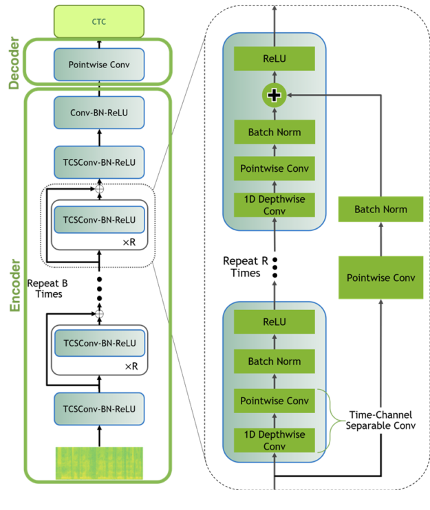"
]
},
{
"cell_type": "markdown",
"metadata": {
"id": "gEpNci7slRzw"
},
"source": [
"# Using NeMo for Automatic Speech Recognition\n",
"\n",
"Now that we have an idea of what ASR is and how the audio data looks like, we can start using NeMo to do some ASR!\n",
"\n",
"We'll be using the **Neural Modules (NeMo) toolkit** for this part, so if you haven't already, you should download and install NeMo and its dependencies. To do so, just follow the directions on the [GitHub page](https://github.com/NVIDIA/NeMo), or in the [documentation](https://docs.nvidia.com/deeplearning/nemo/user-guide/docs/en/stable/).\n",
"\n",
"NeMo lets us easily hook together the components (modules) of our model, such as the data layer, intermediate layers, and various losses, without worrying too much about implementation details of individual parts or connections between modules. NeMo also comes with complete models which only require your data and hyperparameters for training."
]
},
{
"cell_type": "code",
"metadata": {
"id": "4_W0lhaQlRzx"
},
"source": [
"# NeMo's \"core\" package\n",
"import nemo\n",
"# NeMo's ASR collection - this collections contains complete ASR models and\n",
"# building blocks (modules) for ASR\n",
"import nemo.collections.asr as nemo_asr"
],
"execution_count": null,
"outputs": []
},
{
"cell_type": "markdown",
"metadata": {
"id": "v_W8EbYktZE3"
},
"source": [
"## Using an Out-of-the-Box Model\n",
"\n",
"NeMo's ASR collection comes with many building blocks and even complete models that we can use for training and evaluation. Moreover, several models come with pre-trained weights. Let's instantiate a complete QuartzNet15x5 model."
]
},
{
"cell_type": "code",
"metadata": {
"id": "KFZZpYult96G"
},
"source": [
"# This line will download pre-trained QuartzNet15x5 model from NVIDIA's NGC cloud and instantiate it for you\n",
"quartznet = nemo_asr.models.EncDecCTCModel.from_pretrained(model_name=\"QuartzNet15x5Base-En\")"
],
"execution_count": null,
"outputs": []
},
{
"cell_type": "markdown",
"metadata": {
"id": "KucxoFJhum0i"
},
"source": [
"Next, we'll simply add paths to files we want to transcribe into the list and pass it to our model. Note that it will work for relatively short (<25 seconds) files. "
]
},
{
"cell_type": "code",
"metadata": {
"id": "3QCpR_93u1hp"
},
"source": [
"files = [os.path.join(data_dir, 'an4/wav/an4_clstk/mgah/cen2-mgah-b.wav')]\n",
"for fname, transcription in zip(files, quartznet.transcribe(paths2audio_files=files)):\n",
" print(f\"Audio in {fname} was recognized as: {transcription}\")"
],
"execution_count": null,
"outputs": []
},
{
"cell_type": "markdown",
"metadata": {
"id": "ppUm_kuavm_f"
},
"source": [
"That was easy! But there are plenty of scenarios where you would want to fine-tune the model on your own data or even train from scratch. For example, this out-of-the box model will obviously not work for Spanish and would likely perform poorly for telephone audio. So if you have collected your own data, you certainly should attempt to fine-tune or train on it!"
]
},
{
"cell_type": "markdown",
"metadata": {
"id": "ABUDaC5Js7AW"
},
"source": [
"## Training from Scratch\n",
"\n",
"To train from scratch, you need to prepare your training data in the right format and specify your models architecture."
]
},
{
"cell_type": "markdown",
"metadata": {
"id": "RdNyw1b_zgtm"
},
"source": [
"### Creating Data Manifests\n",
"\n",
"The first thing we need to do now is to create manifests for our training and evaluation data, which will contain the metadata of our audio files. NeMo data sets take in a standardized manifest format where each line corresponds to one sample of audio, such that the number of lines in a manifest is equal to the number of samples that are represented by that manifest. A line must contain the path to an audio file, the corresponding transcript (or path to a transcript file), and the duration of the audio sample.\n",
"\n",
"Here's an example of what one line in a NeMo-compatible manifest might look like:\n",
"```\n",
"{\"audio_filepath\": \"path/to/audio.wav\", \"duration\": 3.45, \"text\": \"this is a nemo tutorial\"}\n",
"```\n",
"\n",
"We can build our training and evaluation manifests using `an4/etc/an4_train.transcription` and `an4/etc/an4_test.transcription`, which have lines containing transcripts and their corresponding audio file IDs:\n",
"```\n",
"...\n",
"<s> P I T T S B U R G H </s> (cen5-fash-b)\n",
"<s> TWO SIX EIGHT FOUR FOUR ONE EIGHT </s> (cen7-fash-b)\n",
"...\n",
"```"
]
},
{
"cell_type": "code",
"metadata": {
"id": "lVB1sG1GlRzz"
},
"source": [
"# --- Building Manifest Files --- #\n",
"import json\n",
"\n",
"# Function to build a manifest\n",
"def build_manifest(transcripts_path, manifest_path, wav_path):\n",
" with open(transcripts_path, 'r') as fin:\n",
" with open(manifest_path, 'w') as fout:\n",
" for line in fin:\n",
" # Lines look like this:\n",
" # <s> transcript </s> (fileID)\n",
" transcript = line[: line.find('(')-1].lower()\n",
" transcript = transcript.replace('<s>', '').replace('</s>', '')\n",
" transcript = transcript.strip()\n",
"\n",
" file_id = line[line.find('(')+1 : -2] # e.g. \"cen4-fash-b\"\n",
" audio_path = os.path.join(\n",
" data_dir, wav_path,\n",
" file_id[file_id.find('-')+1 : file_id.rfind('-')],\n",
" file_id + '.wav')\n",
"\n",
" duration = librosa.core.get_duration(filename=audio_path)\n",
"\n",
" # Write the metadata to the manifest\n",
" metadata = {\n",
" \"audio_filepath\": audio_path,\n",
" \"duration\": duration,\n",
" \"text\": transcript\n",
" }\n",
" json.dump(metadata, fout)\n",
" fout.write('\\n')\n",
" \n",
"# Building Manifests\n",
"print(\"******\")\n",
"train_transcripts = data_dir + '/an4/etc/an4_train.transcription'\n",
"train_manifest = data_dir + '/an4/train_manifest.json'\n",
"if not os.path.isfile(train_manifest):\n",
" build_manifest(train_transcripts, train_manifest, 'an4/wav/an4_clstk')\n",
" print(\"Training manifest created.\")\n",
"\n",
"test_transcripts = data_dir + '/an4/etc/an4_test.transcription'\n",
"test_manifest = data_dir + '/an4/test_manifest.json'\n",
"if not os.path.isfile(test_manifest):\n",
" build_manifest(test_transcripts, test_manifest, 'an4/wav/an4test_clstk')\n",
" print(\"Test manifest created.\")\n",
"print(\"***Done***\")"
],
"execution_count": null,
"outputs": []
},
{
"cell_type": "markdown",
"metadata": {
"id": "W2fShQzRzo-M"
},
"source": [
"### Specifying Our Model with a YAML Config File\n",
"\n",
"For this tutorial, we'll build a *Jasper_4x1 model*, with `K=4` blocks of single (`R=1`) sub-blocks and a *greedy CTC decoder*, using the configuration found in `./configs/config.yaml`.\n",
"\n",
"If we open up this config file, we find model section which describes architecture of our model. A model contains an entry labeled `encoder`, with a field called `jasper` that contains a list with multiple entries. Each of the members in this list specifies one block in our model, and looks something like this:\n",
"```\n",
"- filters: 128\n",
" repeat: 1\n",
" kernel: [11]\n",
" stride: [2]\n",
" dilation: [1]\n",
" dropout: 0.2\n",
" residual: false\n",
" separable: true\n",
" se: true\n",
" se_context_size: -1\n",
"```\n",
"The first member of the list corresponds to the first block in the Jasper architecture diagram, which appears regardless of `K` and `R`.\n",
"Next, we have four entries that correspond to the `K=4` blocks, and each has `repeat: 1` since we are using `R=1`.\n",
"These are followed by two more entries for the blocks that appear at the end of our Jasper model before the CTC loss.\n",
"\n",
"There are also some entries at the top of the file that specify how we will handle training (`train_ds`) and validation (`validation_ds`) data.\n",
"\n",
"Using a YAML config such as this is helpful for getting a quick and human-readable overview of what your architecture looks like, and allows you to swap out model and run configurations easily without needing to change your code."
]
},
{
"cell_type": "code",
"metadata": {
"id": "PXVKBniMlRz5"
},
"source": [
"# --- Config Information ---#\n",
"try:\n",
" from ruamel.yaml import YAML\n",
"except ModuleNotFoundError:\n",
" from ruamel_yaml import YAML\n",
"config_path = './configs/config.yaml'\n",
"\n",
"if not os.path.exists(config_path):\n",
" # Grab the config we'll use in this example\n",
" BRANCH = 'r1.17.0'\n",
" !mkdir configs\n",
" !wget -P configs/ https://raw.githubusercontent.com/NVIDIA/NeMo/$BRANCH/examples/asr/conf/config.yaml\n",
"\n",
"yaml = YAML(typ='safe')\n",
"with open(config_path) as f:\n",
" params = yaml.load(f)\n",
"print(params)"
],
"execution_count": null,
"outputs": []
},
{
"cell_type": "markdown",
"metadata": {
"id": "wUmq3p2Aw_5N"
},
"source": [
"### Training with PyTorch Lightning\n",
"\n",
"NeMo models and modules can be used in any PyTorch code where torch.nn.Module is expected.\n",
"\n",
"However, NeMo's models are based on [PytorchLightning's](https://github.com/PyTorchLightning/pytorch-lightning) LightningModule and we recommend you use PytorchLightning for training and fine-tuning as it makes using mixed precision and distributed training very easy. So to start, let's create Trainer instance for training on GPU for 50 epochs"
]
},
{
"cell_type": "code",
"metadata": {
"id": "GUfR6tAK0k2u"
},
"source": [
"import pytorch_lightning as pl\n",
"trainer = pl.Trainer(devices=1, accelerator='gpu', max_epochs=50)"
],
"execution_count": null,
"outputs": []
},
{
"cell_type": "markdown",
"metadata": {
"id": "IEn2RyvgxxvO"
},
"source": [
"Next, we instantiate and ASR model based on our ``config.yaml`` file from the previous section.\n",
"Note that this is a stage during which we also tell the model where our training and validation manifests are."
]
},
{
"cell_type": "code",
"metadata": {
"id": "Cbf0fsMK09lk"
},
"source": [
"from omegaconf import DictConfig\n",
"params['model']['train_ds']['manifest_filepath'] = train_manifest\n",
"params['model']['validation_ds']['manifest_filepath'] = test_manifest\n",
"first_asr_model = nemo_asr.models.EncDecCTCModel(cfg=DictConfig(params['model']), trainer=trainer)"
],
"execution_count": null,
"outputs": []
},
{
"cell_type": "markdown",
"metadata": {
"id": "hWtzwL5qXTYq"
},
"source": [
"With that, we can start training with just one line!"
]
},
{
"cell_type": "code",
"metadata": {
"id": "inRJsnrz1psq"
},
"source": [
"# Start training!!!\n",
"trainer.fit(first_asr_model)"
],
"execution_count": null,
"outputs": []
},
{
"cell_type": "markdown",
"metadata": {
"id": "jpYXX-GslR0E"
},
"source": [
"There we go! We've put together a full training pipeline for the model and trained it for 50 epochs.\n",
"\n",
"If you'd like to save this model checkpoint for loading later (e.g. for fine-tuning, or for continuing training), you can simply call `first_asr_model.save_to(<checkpoint_path>)`. Then, to restore your weights, you can rebuild the model using the config (let's say you call it `first_asr_model_continued` this time) and call `first_asr_model_continued.restore_from(<checkpoint_path>)`.\n",
"\n",
"### After Training: Monitoring Progress and Changing Hyperparameters\n",
"We can now start Tensorboard to see how training went. Recall that WER stands for Word Error Rate and so the lower it is, the better."
]
},
{
"cell_type": "code",
"metadata": {
"id": "n_0y3stSXDX_"
},
"source": [
"try:\n",
" from google import colab\n",
" COLAB_ENV = True\n",
"except (ImportError, ModuleNotFoundError):\n",
" COLAB_ENV = False\n",
"\n",
"# Load the TensorBoard notebook extension\n",
"if COLAB_ENV:\n",
" %load_ext tensorboard\n",
" %tensorboard --logdir lightning_logs/\n",
"else:\n",
" print(\"To use tensorboard, please use this notebook in a Google Colab environment.\")"
],
"execution_count": null,
"outputs": []
},
{
"cell_type": "markdown",
"metadata": {
"id": "Z0h-BME7U8yb"
},
"source": [
"We could improve this model by playing with hyperparameters. We can look at the current hyperparameters with the following:"
]
},
{
"cell_type": "code",
"metadata": {
"id": "7kdQbpohXnEd"
},
"source": [
"print(params['model']['optim'])"
],
"execution_count": null,
"outputs": []
},
{
"cell_type": "markdown",
"metadata": {
"id": "sGZzRCvIW8kE"
},
"source": [
"Let's say we wanted to change the learning rate. To do so, we can create a `new_opt` dict and set our desired learning rate, then call `<model>.setup_optimization()` with the new optimization parameters."
]
},
{
"cell_type": "code",
"metadata": {
"id": "AbigFKUtYgvn"
},
"source": [
"import copy\n",
"new_opt = copy.deepcopy(params['model']['optim'])\n",
"new_opt['lr'] = 0.001\n",
"first_asr_model.setup_optimization(optim_config=DictConfig(new_opt))\n",
"# And then you can invoke trainer.fit(first_asr_model)"
],
"execution_count": null,
"outputs": []
},
{
"cell_type": "markdown",
"metadata": {
"id": "D5Kwg8Cz-aaO"
},
"source": [
"## Inference\n",
"\n",
"Let's have a quick look at how one could run inference with NeMo's ASR model.\n",
"\n",
"First, ``EncDecCTCModel`` and its subclasses contain a handy ``transcribe`` method which can be used to simply obtain audio files' transcriptions. It also has batch_size argument to improve performance."
]
},
{
"cell_type": "code",
"metadata": {
"id": "3FT0klSV268p"
},
"source": [
"paths2audio_files = [os.path.join(data_dir, 'an4/wav/an4_clstk/mgah/cen2-mgah-b.wav'),\n",
" os.path.join(data_dir, 'an4/wav/an4_clstk/fmjd/cen7-fmjd-b.wav'),\n",
" os.path.join(data_dir, 'an4/wav/an4_clstk/fmjd/cen8-fmjd-b.wav'),\n",
" os.path.join(data_dir, 'an4/wav/an4_clstk/fkai/cen8-fkai-b.wav')]\n",
"print(first_asr_model.transcribe(paths2audio_files=paths2audio_files,\n",
" batch_size=4))"
],
"execution_count": null,
"outputs": []
},
{
"cell_type": "markdown",
"metadata": {
"id": "6FiCfLX0D7py"
},
"source": [
"Below is an example of a simple inference loop in pure PyTorch. It also shows how one can compute Word Error Rate (WER) metric between predictions and references."
]
},
{
"cell_type": "code",
"metadata": {
"id": "7mP4r1Gx_Ilt"
},
"source": [
"# Bigger batch-size = bigger throughput\n",
"params['model']['validation_ds']['batch_size'] = 16\n",
"\n",
"# Setup the test data loader and make sure the model is on GPU\n",
"first_asr_model.setup_test_data(test_data_config=params['model']['validation_ds'])\n",
"first_asr_model.cuda()\n",
"first_asr_model.eval()\n",
"\n",
"# We will be computing Word Error Rate (WER) metric between our hypothesis and predictions.\n",
"# WER is computed as numerator/denominator.\n",
"# We'll gather all the test batches' numerators and denominators.\n",
"wer_nums = []\n",
"wer_denoms = []\n",
"\n",
"# Loop over all test batches.\n",
"# Iterating over the model's `test_dataloader` will give us:\n",
"# (audio_signal, audio_signal_length, transcript_tokens, transcript_length)\n",
"# See the AudioToCharDataset for more details.\n",
"for test_batch in first_asr_model.test_dataloader():\n",
" test_batch = [x.cuda() for x in test_batch]\n",
" targets = test_batch[2]\n",
" targets_lengths = test_batch[3] \n",
" log_probs, encoded_len, greedy_predictions = first_asr_model(\n",
" input_signal=test_batch[0], input_signal_length=test_batch[1]\n",
" )\n",
" # Notice the model has a helper object to compute WER\n",
" first_asr_model._wer.update(greedy_predictions, targets, targets_lengths)\n",
" _, wer_num, wer_denom = first_asr_model._wer.compute()\n",
" first_asr_model._wer.reset()\n",
" wer_nums.append(wer_num.detach().cpu().numpy())\n",
" wer_denoms.append(wer_denom.detach().cpu().numpy())\n",
"\n",
" # Release tensors from GPU memory\n",
" del test_batch, log_probs, targets, targets_lengths, encoded_len, greedy_predictions\n",
"\n",
"# We need to sum all numerators and denominators first. Then divide.\n",
"print(f\"WER = {sum(wer_nums)/sum(wer_denoms)}\")"
],
"execution_count": null,
"outputs": []
},
{
"cell_type": "markdown",
"metadata": {
"id": "0kM9kBNOCptf"
},
"source": [
"This WER is not particularly impressive and could be significantly improved. You could train longer (try 100 epochs) to get a better number. Check out the next section on how to improve it further."
]
},
{
"cell_type": "markdown",
"metadata": {
"id": "RBcJtg5ulR0H"
},
"source": [
"## Model Improvements\n",
"\n",
"You already have all you need to create your own ASR model in NeMo, but there are a few more tricks that you can employ if you so desire. In this section, we'll briefly cover a few possibilities for improving an ASR model.\n",
"\n",
"### Data Augmentation\n",
"\n",
"There exist several ASR data augmentation methods that can increase the size of our training set.\n",
"\n",
"For example, we can perform augmentation on the spectrograms by zeroing out specific frequency segments (\"frequency masking\") or time segments (\"time masking\") as described by [SpecAugment](https://arxiv.org/abs/1904.08779), or zero out rectangles on the spectrogram as in [Cutout](https://arxiv.org/pdf/1708.04552.pdf). In NeMo, we can do all three of these by simply adding in a `SpectrogramAugmentation` neural module. (As of now, it does not perform the time warping from the SpecAugment paper.)\n",
"\n",
"Our toy model does not do spectrogram augmentation. But the real one we got from cloud does:"
]
},
{
"cell_type": "code",
"metadata": {
"id": "9glGogaPlR0H"
},
"source": [
"print(quartznet._cfg['spec_augment'])"
],
"execution_count": null,
"outputs": []
},
{
"cell_type": "markdown",
"metadata": {
"id": "LdwdcA_a640R"
},
"source": [
"If you want to enable SpecAugment in your model, make sure your .yaml config file contains 'model/spec_augment' section which looks like the one above."
]
},
{
"cell_type": "markdown",
"metadata": {
"id": "2f142kIQc1Z2"
},
"source": [
"### Transfer learning\n",
"\n",
"Transfer learning is an important machine learning technique that uses a model’s knowledge of one task to make it perform better on another. Fine-tuning is one of the techniques to perform transfer learning. It is an essential part of the recipe for many state-of-the-art results where a base model is first pretrained on a task with abundant training data and then fine-tuned on different tasks of interest where the training data is less abundant or even scarce.\n",
"\n",
"In ASR you might want to do fine-tuning in multiple scenarios, for example, when you want to improve your model's performance on a particular domain (medical, financial, etc.) or on accented speech. You can even transfer learn from one language to another! Check out [this paper](https://arxiv.org/abs/2005.04290) for examples.\n",
"\n",
"Transfer learning with NeMo is simple. Let's demonstrate how the model we got from the cloud could be fine-tuned on AN4 data. (NOTE: this is a toy example). And, while we are at it, we will change model's vocabulary, just to demonstrate how it's done."
]
},
{
"cell_type": "code",
"metadata": {
"id": "hl320dsydWX0"
},
"source": [
"# Check what kind of vocabulary/alphabet the model has right now\n",
"print(quartznet.decoder.vocabulary)\n",
"\n",
"# Let's add \"!\" symbol there. Note that you can (and should!) change the vocabulary\n",
"# entirely when fine-tuning using a different language.\n",
"quartznet.change_vocabulary(\n",
" new_vocabulary=[\n",
" ' ', 'a', 'b', 'c', 'd', 'e', 'f', 'g', 'h', 'i', 'j', 'k', 'l', 'm', 'n',\n",
" 'o', 'p', 'q', 'r', 's', 't', 'u', 'v', 'w', 'x', 'y', 'z', \"'\", \"!\"\n",
" ]\n",
")"
],
"execution_count": null,
"outputs": []
},
{
"cell_type": "markdown",
"metadata": {
"id": "M7lvmiMSd3Aw"
},
"source": [
"After this, our decoder has completely changed, but our encoder (which is where most of the weights are) remained intact. Let's fine tune-this model for 2 epochs on AN4 dataset. We will also use the smaller learning rate from ``new_opt` (see the \"After Training\" section)`."
]
},
{
"cell_type": "code",
"metadata": {
"id": "_PZJIso-eDl-"
},
"source": [
"# Use the smaller learning rate we set before\n",
"quartznet.setup_optimization(optim_config=DictConfig(new_opt))\n",
"\n",
"# Point to the data we'll use for fine-tuning as the training set\n",
"quartznet.setup_training_data(train_data_config=params['model']['train_ds'])\n",
"\n",
"# Point to the new validation data for fine-tuning\n",
"quartznet.setup_validation_data(val_data_config=params['model']['validation_ds'])\n",
"\n",
"# And now we can create a PyTorch Lightning trainer and call `fit` again.\n",
"trainer = pl.Trainer(devices=1, accelerator='gpu', max_epochs=2)\n",
"trainer.fit(quartznet)"
],
"execution_count": null,
"outputs": []
},
{
"cell_type": "markdown",
"metadata": {
"id": "VURa1NavlR0U"
},
"source": [
"### Fast Training\n",
"\n",
"Last but not least, we could simply speed up training our model! If you have the resources, you can speed up training by splitting the workload across multiple GPUs. Otherwise (or in addition), there's always mixed precision training, which allows you to increase your batch size.\n",
"\n",
"You can use [PyTorch Lightning's Trainer object](https://pytorch-lightning.readthedocs.io/en/latest/common/trainer.html?highlight=Trainer) to handle mixed-precision and distributed training for you. Below are some examples of flags you would pass to the `Trainer` to use these features:\n",
"\n",
"```python\n",
"# Mixed precision:\n",
"trainer = pl.Trainer(amp_level='O1', precision=16)\n",
"\n",
"# Trainer with a distributed backend:\n",
"trainer = pl.Trainer(devices=2, num_nodes=2, accelerator='gpu', strategy='ddp')\n",
"\n",
"# Of course, you can combine these flags as well.\n",
"```\n",
"\n",
"Finally, have a look at [example scripts in NeMo repository](https://github.com/NVIDIA/NeMo/blob/stable/examples/asr/asr_ctc/speech_to_text_ctc.py) which can handle mixed precision and distributed training using command-line arguments."
]
},
{
"cell_type": "markdown",
"metadata": {
"id": "d1ym8QT3jQnj"
},
"source": [
"### Deployment\n",
"\n",
"Note: It is recommended to run the deployment code from the NVIDIA PyTorch container.\n",
"\n",
"Let's get back to our pre-trained model and see how easy it can be exported to an ONNX file\n",
"in order to run it in an inference engine like TensorRT or ONNXRuntime.\n",
"\n",
"If you are running in an environment outside of the NVIDIA PyTorch container (like Google Colab for example) then you will have to build the onnxruntime and onnxruntime-gpu. The cell below gives an example of how to build those runtimes but the example may have to be adapted depending on your environment."
]
},
{
"cell_type": "code",
"metadata": {
"id": "I4WRcmakjQnj"
},
"source": [
"!pip install --upgrade onnxruntime # for gpu, use onnxruntime-gpu\n",
"#!mkdir -p ort\n",
"#%cd ort\n",
"#!git clean -xfd\n",
"#!git clone --depth 1 --branch v1.8.0 https://github.com/microsoft/onnxruntime.git .\n",
"#!./build.sh --skip_tests --config Release --build_shared_lib --parallel --use_cuda --cuda_home /usr/local/cuda --cudnn_home /usr/lib/#x86_64-linux-gnu --build_wheel\n",
"#!pip uninstall -y onnxruntime\n",
"#!pip uninstall -y onnxruntime-gpu\n",
"#!pip install --upgrade --force-reinstall ./build/Linux/Release/dist/onnxruntime*.whl\n",
"#%cd .."
],
"execution_count": null,
"outputs": []
},
{
"cell_type": "markdown",
"metadata": {
"id": "F9yO1BEbjQnm"
},
"source": [
"Then run"
]
},
{
"cell_type": "code",
"metadata": {
"id": "HZnyWxPyjQnm"
},
"source": [
"import json\n",
"import os\n",
"import tempfile\n",
"import onnxruntime\n",
"import torch\n",
"\n",
"import numpy as np\n",
"import nemo.collections.asr as nemo_asr\n",
"from nemo.collections.asr.data.audio_to_text import AudioToCharDataset\n",
"from nemo.collections.asr.metrics.wer import WER\n",
"\n",
"def to_numpy(tensor):\n",
" return tensor.detach().cpu().numpy() if tensor.requires_grad else tensor.cpu().numpy()\n",
"\n",
"def setup_transcribe_dataloader(cfg, vocabulary):\n",
" config = {\n",
" 'manifest_filepath': os.path.join(cfg['temp_dir'], 'manifest.json'),\n",
" 'sample_rate': 16000,\n",
" 'labels': vocabulary,\n",
" 'batch_size': min(cfg['batch_size'], len(cfg['paths2audio_files'])),\n",
" 'trim_silence': True,\n",
" 'shuffle': False,\n",
" }\n",
" dataset = AudioToCharDataset(\n",
" manifest_filepath=config['manifest_filepath'],\n",
" labels=config['labels'],\n",
" sample_rate=config['sample_rate'],\n",
" int_values=config.get('int_values', False),\n",
" augmentor=None,\n",
" max_duration=config.get('max_duration', None),\n",
" min_duration=config.get('min_duration', None),\n",
" max_utts=config.get('max_utts', 0),\n",
" blank_index=config.get('blank_index', -1),\n",
" unk_index=config.get('unk_index', -1),\n",
" normalize=config.get('normalize_transcripts', False),\n",
" trim=config.get('trim_silence', True),\n",
" parser=config.get('parser', 'en'),\n",
" )\n",
" return torch.utils.data.DataLoader(\n",
" dataset=dataset,\n",
" batch_size=config['batch_size'],\n",
" collate_fn=dataset.collate_fn,\n",
" drop_last=config.get('drop_last', False),\n",
" shuffle=False,\n",
" num_workers=config.get('num_workers', 0),\n",
" pin_memory=config.get('pin_memory', False),\n",
" )\n",
"\n",
"quartznet = nemo_asr.models.EncDecCTCModel.from_pretrained(model_name=\"QuartzNet15x5Base-En\")\n",
"\n",
"quartznet.export('qn.onnx')\n",
"\n",
"ort_session = onnxruntime.InferenceSession('qn.onnx', providers=['TensorrtExecutionProvider', 'CUDAExecutionProvider', 'CPUExecutionProvider'])\n",
"\n",
"with tempfile.TemporaryDirectory() as tmpdir:\n",
" with open(os.path.join(tmpdir, 'manifest.json'), 'w') as fp:\n",
" for audio_file in files:\n",
" entry = {'audio_filepath': audio_file, 'duration': 100000, 'text': 'nothing'}\n",
" fp.write(json.dumps(entry) + '\\n')\n",
"\n",
" config = {'paths2audio_files': files, 'batch_size': 4, 'temp_dir': tmpdir}\n",
" temporary_datalayer = setup_transcribe_dataloader(config, quartznet.decoder.vocabulary)\n",
" for test_batch in temporary_datalayer:\n",
" processed_signal, processed_signal_len = quartznet.preprocessor(\n",
" input_signal=test_batch[0].to(quartznet.device), length=test_batch[1].to(quartznet.device)\n",
" )\n",
" ort_inputs = {ort_session.get_inputs()[0].name: to_numpy(processed_signal),}\n",
" ologits = ort_session.run(None, ort_inputs)\n",
" alogits = np.asarray(ologits)\n",
" logits = torch.from_numpy(alogits[0])\n",
" greedy_predictions = logits.argmax(dim=-1, keepdim=False)\n",
" wer = WER(decoding=quartznet.decoding, use_cer=False)\n",
" hypotheses, _ = wer.decoding.ctc_decoder_predictions_tensor(greedy_predictions)\n",
" print(hypotheses)\n",
" break\n"
],
"execution_count": null,
"outputs": []
},
{
"cell_type": "markdown",
"metadata": {
"id": "wteGqroafWg1"
},
"source": [
"## Under the Hood\n",
"\n",
"NeMo is open-source and we do all our model development in the open, so you can inspect our code if you wish.\n",
"\n",
"In particular, ``nemo_asr.model.EncDecCTCModel`` is an encoder-decoder model which is constructed using several ``Neural Modules`` taken from ``nemo_asr.modules.`` Here is what its forward pass looks like:\n",
"```python\n",
"def forward(self, input_signal, input_signal_length):\n",
" processed_signal, processed_signal_len = self.preprocessor(\n",
" input_signal=input_signal, length=input_signal_length,\n",
" )\n",
" # Spec augment is not applied during evaluation/testing\n",
" if self.spec_augmentation is not None and self.training:\n",
" processed_signal = self.spec_augmentation(input_spec=processed_signal)\n",
" encoded, encoded_len = self.encoder(audio_signal=processed_signal, length=processed_signal_len)\n",
" log_probs = self.decoder(encoder_output=encoded)\n",
" greedy_predictions = log_probs.argmax(dim=-1, keepdim=False)\n",
" return log_probs, encoded_len, greedy_predictions\n",
"```\n",
"Here:\n",
"\n",
"* ``self.preprocessor`` is an instance of ``nemo_asr.modules.AudioToMelSpectrogramPreprocessor``, which is a neural module that takes audio signal and converts it into a Mel-Spectrogram\n",
"* ``self.spec_augmentation`` - is a neural module of type ```nemo_asr.modules.SpectrogramAugmentation``, which implements data augmentation. \n",
"* ``self.encoder`` - is a convolutional Jasper/QuartzNet-like encoder of type ``nemo_asr.modules.ConvASREncoder``\n",
"* ``self.decoder`` - is a ``nemo_asr.modules.ConvASRDecoder`` which simply projects into the target alphabet (vocabulary).\n",
"\n",
"Also, ``EncDecCTCModel`` uses the audio dataset class ``nemo_asr.data.AudioToCharDataset`` and CTC loss implemented in ``nemo_asr.losses.CTCLoss``.\n",
"\n",
"You can use these and other neural modules (or create new ones yourself!) to construct new ASR models."
]
},
{
"cell_type": "markdown",
"metadata": {
"id": "smzlvbhelR0U"
},
"source": [
"# Further Reading/Watching:\n",
"\n",
"That's all for now! If you'd like to learn more about the topics covered in this tutorial, here are some resources that may interest you:\n",
"- [Stanford Lecture on ASR](https://www.youtube.com/watch?v=3MjIkWxXigM)\n",
"- [\"An Intuitive Explanation of Connectionist Temporal Classification\"](https://towardsdatascience.com/intuitively-understanding-connectionist-temporal-classification-3797e43a86c)\n",
"- [Explanation of CTC with Prefix Beam Search](https://medium.com/corti-ai/ctc-networks-and-language-models-prefix-beam-search-explained-c11d1ee23306)\n",
"- [Listen Attend and Spell Paper (seq2seq ASR model)](https://arxiv.org/abs/1508.01211)\n",
"- [Explanation of the mel spectrogram in more depth](https://towardsdatascience.com/getting-to-know-the-mel-spectrogram-31bca3e2d9d0)\n",
"- [Jasper Paper](https://arxiv.org/abs/1904.03288)\n",
"- [QuartzNet paper](https://arxiv.org/abs/1910.10261)\n",
"- [SpecAugment Paper](https://arxiv.org/abs/1904.08779)\n",
"- [Explanation and visualization of SpecAugment](https://towardsdatascience.com/state-of-the-art-audio-data-augmentation-with-google-brains-specaugment-and-pytorch-d3d1a3ce291e)\n",
"- [Cutout Paper](https://arxiv.org/pdf/1708.04552.pdf)\n",
"- [Transfer Learning Blogpost](https://developer.nvidia.com/blog/jump-start-training-for-speech-recognition-models-with-nemo/)"
]
},
{
"cell_type": "code",
"metadata": {
"id": "V3ERGX86lR0V"
},
"source": [],
"execution_count": null,
"outputs": []
}
]
}
|